
Generation and Transformation of Representations
This chapter gives some basic methods for generating new representations and for transforming a given representation into another representation. The generation and transformation of representations can be regarded as procedures for creating output that is represented differently from the one used as input. Each method depends on the type of representation used. We will describe the linear transformation of patterns, the generation of spatial structure representations, the generation of trees, problem solving by heuristic search, inference in predicate logic, inference using rules, and inference using frames. These methods, along with those in Chapter 2, are the fundamental techniques needed to understand Chapter 4 and later chapters. There are many methods for the generation and transformation of representations. What we describe in this chapter are examples of these methods.
3.1 Methods of Generating and Transforming Representations
The generation and transformation of different representations can be thought of as procedures for creating output information whose form of representation is different from that of the input information. “Generation” and “transformation” are not very different. We call the process “generation” when we direct our attention to a newly created form of representation and “transformation” when we are interested in the process of making one representation from another.
[Example Problem] Suppose we have the two-dimensional bit pattern shown in Figure 3.1. Transform this so that it is represented by a spatial structure. Also transform it into a graph.
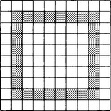
We represent the two-dimensional bit pattern in Figure 3.1 using the set A = {f(x, y)|0 ≤ x ≤ 9,0 ≤ y ≤ 9, x, y integer}. In A, when a point (x, y) corresponds to ![]() , we let f(x, y) = 1, and when it corresponds to
, we let f(x, y) = 1, and when it corresponds to ![]() , we let f(x, y) = 0. The only set of four points such that f(x, y) = f(x · 1, y) = f(x, y · 1) = 1 (where · is + or -) is (1, 1), (1, 8), (8, 1), (8, 8). We can see that by simply checking each point, (x, y), where f(x, y) = 1. A little thought will show that this criterion uniquely determines a square. Another way of looking at this is to consider the points that can be reached by changing only either one of the x and y coordinates. For example, the four points (1, 1), (8, 1), (8, 8), (1,8) are in this order. We can write this as B = ((1, 1), (8, 1), (8, 8), (1, 8)). Here B is the spatial structure representation described in Section 2.2 that results from transforming the original representation A.
, we let f(x, y) = 0. The only set of four points such that f(x, y) = f(x · 1, y) = f(x, y · 1) = 1 (where · is + or -) is (1, 1), (1, 8), (8, 1), (8, 8). We can see that by simply checking each point, (x, y), where f(x, y) = 1. A little thought will show that this criterion uniquely determines a square. Another way of looking at this is to consider the points that can be reached by changing only either one of the x and y coordinates. For example, the four points (1, 1), (8, 1), (8, 8), (1,8) are in this order. We can write this as B = ((1, 1), (8, 1), (8, 8), (1, 8)). Here B is the spatial structure representation described in Section 2.2 that results from transforming the original representation A.
Let us now transform the representation B into a graph representation. Suppose we write B in the form (b1, b2, b3,b4) and represent the relation that a point in B is “next to” another point by the label “neighbor.” When each of bi (i = 1,…, 4) is a node and bi+1 is next to bi, and if we define the directed edge from bi to bi+1 and give it the label “neighbor,” we obtain the graph shown in Figure 3.2. If we call this graph C, C is a graph representation obtained by transforming B.
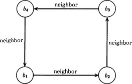
Figure 3.2 A graph representation of Figure 3.1.
The example above shows a particular transformation method that is closely tied only to this example. In the following sections, we will look at more general methods for transforming various representations.
3.2 Linear Transformations of Pattern Functions
A pattern function defined on a continuous domain usually includes noise and is based on incomplete data. In such a case, it may be more convenient to transform it into some other function in order to find some additional information or structure in a form of the new function. Among the methods for transforming a pattern function on a continuous domain to another function, we first describe the use of linear transformations.
Throughout this book, we will omit detailed descriptions of assumptions that need to be made about the functions we are looking at. These include the continuity, differentiability, and boundedness of functions as well as the cardinality of the set of local maxima and minima of the functions. Basically, we assume that what we describe in this book will be true for functions that are bounded, second-order differentiable, and satisfy appropriate boundary conditions.
(a) Convolution integral
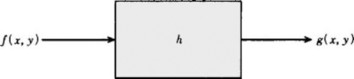
First, we describe the following simple method of transforming a pattern function. Let us consider the situation where a pattern function f(x, y) is transformed into another pattern function g(x, y) using the transformation h shown in Figure 3.3. In other words, g(x, y) = h(f(x, y)).
Let us also assume that the following property is true for x and y in the two pattern functions, f1(x, y) and f2(x, y), for some real constants r and s:
A transformation h with this property is called a linear transformation. We now look at the function δ(x, y) with the following property:
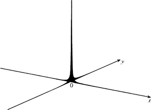
The function with such characteristics is generally called the (two-dimensional) delta function (δ function). The intuitive form of the delta function is illustrated in Figure 3.4.
Using the definition above, we can represent the transformation h using the delta function. First, we can obtain the value of f(x, y) at the point (a, b) by evaluating
In this equation, a, b and x, y can be exchanged. Namely,
Also, we let
This ϕ is called the point spread function or the impulse response of the transformation h. It is called a point spread function because a function with a value only at one point like the delta function in Figure 3.4 can “spread” its value through the transformation h. The point spread function ϕ is obtained by using the function h to transform the delta function that takes the value ∞ only at the point (x, y) = (a, b). We are assuming here that ϕ has the same form independent of the location of (a, b). In other words, we assume that ϕ(x, y, a, b) can always be expressed as ϕ(x-a, y-b). Such a ϕ is called a shift-invariant point spread function
When ϕ is a shift-invariant point spread function, we have
In equation (3.2), intuitively, the function g(x, y), which is the result of transforming the function f(x, y) using h, represents the sum of the product of the original function f(x, y) and the point spread function ϕ(a, b) while keeping x and y fixed and varying a and b. Generally, an integral of the form
or, in two-dimensional form, a double integral
is called a convolution integral and is written p(x) * q(x) or p(x, y) * q(x, y). Using this convolution integral, equation (3.2) can be written
Thus the new pattern g that can be obtained by applying the linear transformation formation h to f will be a convolution integral of f and a point spread function ϕ.
(b) Fourier transform
Although the convolution integral is an important method of performing a linear transformation on a pattern function, it is sometimes difficult to calculate the integral. Instead we can transform the convolution integral over a spatial domain (x, y) to a representation in another domain, do the calculation in that space, and retransform the result to the original (x, y) space. The frequency domain is often used for the alternative domain. We will now explain the Fourier transform as such a transformation.
If we rewrite equation (2.1) for the Fourier transform described in Section 2.12 into the complex function form using the Euler formula
where j2 = −1, we get
Therefore, we generally obtain the following:
If
we will get the following from expressions (3.3)–(3.6):
If we make L → ∞ and thus Δω → 0, under appropriate conditions, we will get
Expression (3.7) is called the Fourier integral. If we make
(3.7) can be rewritten as
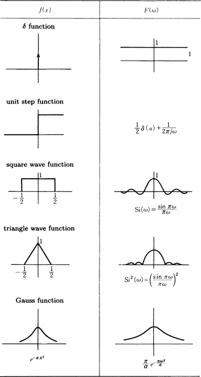
Equation (3.8) is called a Fourier transform and equation (3.9) is called an inverse Fourier transform. Figure 3.5 shows an example of a Fourier transform.
So far we have used functions of one variable. Let us extend our representation to include functions of two variables and, at the same time, make the appropriate variable transformation. Using the function exp(-2πj(ux + vy)) on the two-dimensional frequency domain (u, v), the function f(x, y) on the spatial domain (x, y) can be transformed to the following function in the frequency domain:
This transformation is one of the forms for the (two-dimensional) Fourier transform, u and v are called the spatial frequencies. The Fourier transform F(f(u, v) for f(x, y) is written f(x, y)).
The transform from the frequency domain to the spatial domain can be defined as
This transform is the (two-dimensional) inverse Fourier transform. The inverse Fourier transform of F(u, v) is written F−1(F(u, v)).
There are many relations between the Fourier transform or the inverse Fourier transform and the convolution integral. One of them is the following convolution theorem.
Theorem 1
(convolution theorem). The Fourier transform of the product of two functions, f(x, y) and g(x, y), is equal to the product of the Fourier transforms F(u, v) and G(u, v). In other words,
If we take the inverse Fourier transform of both sides of expression (3.12), then, by Theorem 1, we get the following:
In other words,
So, if we take the Fourier transforms for two functions in the spatial domain, take the product of them, and take the inverse Fourier transform of the result, we will obtain the convolution integral of the original functions.
Fourier transforms also have the following properties: If we perform a linear transformation of the function exp(2πj(ux + vy)) by the convolution using the transformation ft, we will get the following:
where
The above result shows that a linear transformation of exp(2πj(ux + vy)) is the product of the Fourier transforms of the point spread function ϕ, Φ(u, v), and the original function, exp(27πj(ux + vy)). Generally, exp(2πj(uv + vy)) is called an eigenfunction of the linear transformation h, and Φ(u, v) is called its eigenvalue.
3.3 Sampling and Quantization of Pattern Functions
(a) Sampling
As we observed in Section 2.1, a pattern function can be represented on a continuous domain or can be a discrete representation such as a bit array. In this section we explore how to approximate a pattern function on a continuous domain by a discrete function on a quantized domain.
To simplify, we will consider only functions f(x) on the real line as the pattern functions on a continuous domain. Further, we assume that f(x) can be represented approximately by a comb-shaped function with interval Δx, as shown in Figure 3.6.
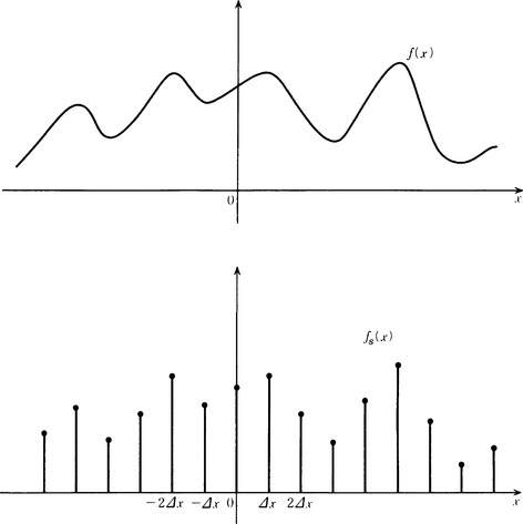
Taking the value of a function defined on a continuous domain only at discrete points, as described in Section 2.1, is called sampling the function. If we let fs(x) be the function that takes those sampling points as its domain, then for integer n we have
If we take the Fourier transform of both sides, we get
by using ![]() . Expression (3.13) shows that the sampling of f(x) takes the sum in the interval 1/Δx for the Fourier transform of f(x).
. Expression (3.13) shows that the sampling of f(x) takes the sum in the interval 1/Δx for the Fourier transform of f(x).
When ![]() , we assume that the value of F(u) is always 0. (We say that such an F(u) is bandlimited.) In this case, the inverse Fourier transform
, we assume that the value of F(u) is always 0. (We say that such an F(u) is bandlimited.) In this case, the inverse Fourier transform
multiplied by fs(u) is equal to the original function f(x). In other words,
All of these results can be collected in a theorem called the sampling theorem.
Theorem 2
(sampling theorem). If the Fourier transform of a pattern function does not include more than half of the spatial frequency component of the sampled frequency, we can reconstruct the original function on the spatial domain from the sampling values in the frequency domain.
According to the sampling theorem, if the Fourier transform F(u) of the original function f(x) does not include high-frequency components, the transformation by sampling is sufficiently effective. Although this condition seems to be too strict, it is possible to make it work in the real world if we preprocess the high-frequency components of F(u) using a low-pass filter.
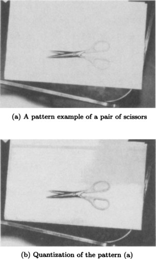
(b) Quantization
The purpose of sampling as described in (a) is to discretize the domain of a pattern function. On the other hand, segmenting the values of a function, as we described in Section 2.1, is called quantization. Quantization is done by limiting the value of a function to only a few quantization levels. For example, Figure 3.7(b) shows quantization into three-bit levels for the pattern shown in Figure 3.7(a).
In order to generate a one-bit quantization pattern, ![]() , for a pattern function f(x), we first obtain the frequency distribution of the intensity values of the pattern elements of f(x). We then let α be the minimum intensity in the distribution and make
, for a pattern function f(x), we first obtain the frequency distribution of the intensity values of the pattern elements of f(x). We then let α be the minimum intensity in the distribution and make
3.4 Transformation to Spatial Representations
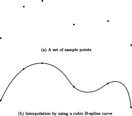
There are many methods for generating spatial representations from a pattern function. Chapter 4 will provide several popular methods. In this section, we will describe one example, a method for creating a curve by interpolating points, which are given as a set of sampled points. This problem occurs when we try to infer the boundary line or the region of an incomplete pattern. Let us consider the set of sample points shown in Figure 3.8(a). How could we approximate a path through these points that is as smooth as possible? As a method for the approximation, here we will describe spline function approximation, in particular the B-spline function method.
We define the curve going through n sample points, a1,…, an, as follows using the parameter s:
To simplify, we assume ai = a(i) (i = 1,…,n). We also assume that each interval (i, i +1) (i = 1,…, n−1) has the same length along s. Furthermore, we assume
for the coefficient bk (k = 0,1,…, n + 1). These are boundary conditions that the curvatures at the end points a and an are 0.
Our purpose is to find a curve, ai(s) (i = 1,…, n− 1), for connecting two neighboring points ai and ai+1 in the form of expression (3.14). Suppose each ai(s) is represented as a cubic polynomial function. (The method of using a cubic polynomial function is called the cubic B-spline method.) This can be done in the following way:
We assume that the function Bk(s) (k = 0,1,…, n + 1) on the right side of (3.14) takes only nonnegative values, and it may not be 0 only on the four curved parts between (ak−2, ak+2)- In other words, for the curve ak(s), only ![]() have nonnegative values. We can determine the coordinates ak(s*) of the point s* within the kth interval (ak,ak+1) as follows:
have nonnegative values. We can determine the coordinates ak(s*) of the point s* within the kth interval (ak,ak+1) as follows:
where

It is known that, using this method, we can obtain a curve that has a continuous second-order derivative at the original sample points ai (i = 1,…, n). We can obtain the curve shown in Figure 3.8(b) at the sample points of Figure 3.8(a). A cubic B-spline is often used as a method of approximating curves, but from the viewpoint of a method of transforming representations, we can consider it a method for creating a curve, which is a spatial structure representation, from the coordinate representation of discrete points. The method we described in this section is just one of many possible methods. We will give some more of them in Chapter 4.
3.5 Generation of Tree Representation
So far we have explained methods for transforming a pattern function to other representations. In this section we will describe a simple method for generating a tree representation as one example of a method for creating a symbolic representation.
Let us consider the problem of discriminating between two lists. In the lists (a b c) and (a c d), the first element of both lists is a, but the second elements, or the third, of these lists are different. In order to discriminate between these two lists, we need only check whether the second element is b or not. This can be represented as the tree shown in Figure 3.9(a). In this tree, node 0 has the procedure “if the second element is b, then output T. Otherwise, output F.” Notice that nodes 1 and 2, which are leaves, correspond to the lists. For a given list, if we start from the root of the tree, execute the procedure at any node we pass, go along the edge labeled with the output, and look at the leaf we reach, we can discriminate between lists. For example, if the given list is (a b c), the output of the procedure at node 0 is T and, as a result, when we reach node 1 we can decide that the list is (a b c).
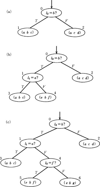
Now, suppose we have the list (e b f). If we execute the procedure above for this list and the tree shown in Figure 3.9(a), we will also reach node 1. As a result, (e b f) will be decided to be the list at node 1, that is (a b c). Since this decision is wrong, we need to delete the list (a b c) from node 1 and add a new procedure for discriminating between (a b c) and (e b f). Let us make the new procedure “if the first element is a, then output T. Otherwise, output F.” Also, we need to generate new nodes 3 and 4 as subnodes of node 2 and let the new nodes have the lists (a b c) and (e b f), respectively. Further, we need to label the edge from node 1 to node 3 with T and the edge from 1 to 4 with F. What we get is the tree shown in Figure 3.9(b). Now let us give the list (e b g) to the tree shown in Figure 3.9(b). As before, we assign the new procedure “if the third element is f, output T. Otherwise output F” to node 4. As a result, we generate a new tree with two new nodes 5 and 6 as subnodes of 4. We show the result in Figure 3.9(c).
Such a tree is called a (binary) discrimination tree for lists. We can summarize the algorithm for generating a discrimination tree for lists as follows, where the lists will be presented in the order L1, L2,…:
Algorithm 3.1
(generation of a discrimination tree for lists)
[1] Generate the root node no.
[2] If the first element of L1 is l1, let no be assigned the procedure “If the first element is l1, output T. Otherwise, output F.”
[3] Generate n1,n2 as subnodes of no and let L1 be assigned to n1. Also, let the symbol “fail” be assigned to node n2.
[4] Call The Tree Obtained In [3] G. Let i = 2. When a node nj has an associated list, call the list L(nj).
[5] Assign Li to the root node no of G, execute the procedure assigned to this node, determine the edge to follow from the output obtained, and go to the appropriate subnode. Repeat this operation. Call the leaf we reach ![]() If Li is already known and we are in the middle of generating the rest of the tree, go to [6]. If Li is unknown and we are discriminating Li, go to [7].
If Li is already known and we are in the middle of generating the rest of the tree, go to [6]. If Li is unknown and we are discriminating Li, go to [7].
[6] If Li does not match L(ni*), do the following substeps (to generate the discrimination tree). When the substeps are done, go to [8].
[6.1] Generate a procedure for discriminating Li and L(ni*). The procedure should receive LiLi and L(ni*) as inputs and output T when the test isolates Li. Otherwise, it should output F.
[6.2] Generate nm+1 and nm+2, the subnodes of (ni*). (We assume that the number for the node created most recently was nm.) Let L(nm+1) = L(ni, nm+2 = L(ni*) and remove L(ni*) from (ni*).
[6.3] Generate an edge from ni* to nm+1 and label it T. Also, generate an edge from ni* to nm+2 and label it F.
[7] Assume that Li is the list to be assigned to ni* and go to [8] (make use of the discrimination tree.)
[8] If there are no lists left, stop. If there is a list remaining, let i = i +1 and go to [5].
This method of generating a discrimination tree for lists can be thought of as a method for transforming a representation of a set of lists into a representation using a tree. In this section, we described how to discriminate lists. By improving the way we decide what procedure to use at each node, we can use a discrimination tree for many different kinds of objects. We will describe some more examples in Chapter 9.
3.6 Search and Problem Solving
(a) Search
So far we have explained several examples of the methods used for transforming one representation into another. We should note that a procedure used for generating a new representation is itself described using a procedural representation. In this section we will explain search, a popular method for finding procedures to attain a goal.
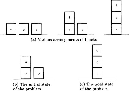
Suppose we have some arrangements of three blocks on a table as shown in Figure 3.10(a). Each possible arrangement can be regarded as a spatial structure representation of a thing we could call “three blocks and a table.” Let us generate a procedure for generating a new arrangement from a given arrangement. We assume that we can ignore the relative left/right positions of the blocks.
(1) One arrangement is given. We call this the initial state.
(2) The arrangement to reach in the end is given. We call this the goal state.
(3) There is a procedure for transforming one state into another.
(4) There is a way to calculate the appropriateness of each state.
that represents the arrangement shown in Figure 3.10(b) is given as the initial state. Let us call the initial state so. Also, the list
that represents the arrangement shown in Figure 3.10(c) is given as the goal state. Let us call it sd..
Let the following three production rules represent the procedure for transforming one state into another:
where $x, $y, and $z are variables that can be replaced by the names of specific blocks. Also, *delete is the procedure for deleting an element of the currently considered list, and *add is the procedure for adding an element to this list as its last element. For example, we can interpret the first rule as
“If the currently considered list includes both (cleartop $x) and (on $x delete (on $x $y), and add (cleartop $y) and (ontable $x) in this order.”
In other words, this rule represents the procedure for “If there is nothing on the block $x, and $x is on $y, remove $x from $y and put it on the table.
This procedure will be executed only when the currently considered list includes both elements (cleartop $x) and (on $x $y). The other two rules can be interpreted similarly.
Using the rules above, we can directly transform one arrangement of blocks into another.
Furthermore, let us define the appropriateness of an arrangement, s, for blocks x and y by the following, where so and sd are the initial and goal states, respectively:
(1) Let f(5) be the number of lists that are included both in s and in sd.
(2) Let g(s) be the number of lists that are of the form (on x y) and are included in s but not in sd.
(3) Let h(s) be the number of lists that are of the form (cleartop x) or (ontable x) and are included in s but not in sd.
(4) Let k(s) be the number of lists that are included in Sd but not in s.
For example, the appropriateness of the initial arrangement, so, is
Now, we start from the initial state, so, execute each of the three production rules whose condition side matches the currently considered list to generate a new state, and repeat the execution until we reach the goal state.
Usually, more than one rule can be executed to produce a new state. For example, if we search all the states that can be generated from the initial state, we will generate the tree shown in Figure 3.11. In Figure 3.11, the number attached to each state represents its appropriateness computed using the above definition.
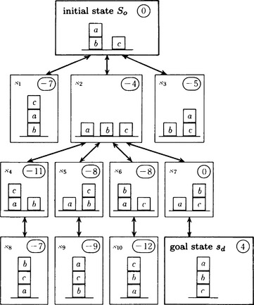
We call a tree like the one in Figure 3.11 a search tree and the method of search that generates a search tree a tree search. In Figure 3.11, the path from so to sd is the path passing through the states so, s2, s7, sd. If we list the rules that were executed in generating this path, such a list would be a representation of the procedures for generating the goal state, sd, from the initial state, s.o
There are many methods for generating a tree like the one shown in Figure 3.11. We will give some more later. Before we do that, we need to formalize what we have explained so far. In particular, the search described above is actually a kind of representation transformation called problem solving. Now we briefly describe problem solving.
(b) Problem solving
We view each arrangement of the blocks shown in (a) as a state and call the collection of possible arrangements the state space. Searching for a path from the initial state so to the goal state sd is equivalent to searching for a sequence of states starting from the initial state and reaching the goal state in a given state space. Moving from one state to another is called state transition, and the procedure for making a state transition is applying a state transition operator to the present state. A state transition can be defined as a rule for taking the pair of a state and an operator and making it correspond to the state that is moved to. Such a rule is called a state transition rule.
Suppose we have a state space S, a set of operators A, a set of state transition rules M, the initial state so, and the goal state sd, both in S. We call the tuple of these five elements P = 〈S, A, M, so, sd〉 a problem. Sometimes an operator and a state transition rule can be identified. In such a case this definition is redundant.
For a problem P, to find a sequence of operators that will move so to sd is called problem solving, and an obtained sequence of operators is called a solution to P. For example, the arrangement of the blocks shown in (a) can be considered to be a problem if we make the following definitions:
(1) Let a possible arrangement of the blocks be a state and the set of all such arrangements the state space S.
(2) Let A = {r1,r2, r3} be the set of operators, where r1, r2, and r3 are the three rules shown in (3), respectively.
(3) Suppose we have a state s ∈ S and a rule ri that can be applied to that state. If we apply rito s, we obtain another state s′. This state transition can be defined as the rule ri : s ⇐ s′. We regard such a rule as a state transition rule and call the set of all possible such rules the set M of state transition rules.
(4) Let the initial arrangement so given in (a) be the initial state so.
(5) Let the goal arrangement sd in (a) be the goal state sdSd>
(6) Based on (1)-(5), we define the problem P = 〈S, A, M, sd, sd〉>
Generating a procedural representation that corresponds to a path from so to sd shown in the example (a) is the same as obtaining a sequence of operators for generating a path from so to sd in the problem P.
In this example, we used lists to represent information. There are many other methods for representing S, A, M, so, sd, and P.
(c) Depth-first search
As we noted, in general there may be more than one state that can be reached from a state s in the state space. Thus, the following algorithm can be used as a search method: First, pick a state that can be reached from s but has not been visited before, and move to such a state s′. Then, pick and move to another such possible state. Repeat this operation until we reach the goal state sd. If there is no state that can be reached from s and has never been visited before, go one step backward from s and search down another possible state that can be reached from s. This backward-step procedure in the search is called backtracking.
Using this algorithm, the direction of the search usually goes in a deeper direction from the initial state, so this kind of algorithm is called depth-first search. This search method is well-adapted to finding a deeper path, or a long route, but it can take a long time to reach the goal when you go deep into one direction but the goal state lies in a different direction.
We now show the most basic algorithm for depth-first search.
Algorithm 3.2
[1] Let s = so, Z = {so}, Q = ( ), sb = ( ).
[2] If s = sd then stop. The sequence of operators given in Q is a solution. Otherwise, go to [3].
[3] Find a state that can be directly reached from ss but is not included in Z, and call it s′. Let Z = Z ∪ {s′}. For a(s, s′), an operator for moving s′ to s′, add the new element a(s,s) to the front of the list Q. Let the new list be Q and go to [4]. If such an s′ does not exist, go to [5].
[4] Let s = s′. Add the new element ss to the front of the list sb, and let the new list be Go to [2].
[5] If sb = ( ), then stop. There is no solution. Otherwise, let s be the first element (s1) of the list Delete s1 from sb and let sb be the list sb without s.1 Furthermore, delete the first element of Q, a(s1, s), from Q and let the new list be Q. Go to [3].
If we use Algorithm 3.2 on the example shown in (a), we will obtain the following state transitions in Figure 3.11 starting from so:
(d) Breadth-first search
The method of depth-first search repeats the process of searching only one state that is directly accessible and has not been searched before. Thus, the search goes deeper and deeper. On the other hand, breadth-first search is a method that tries to search all states that are directly accessible and have not been searched, before going down deeper. Unlike depth-first search, an algorithm for breadth-first search does not include a procedure for backtracking. Instead, it may take longer to solve a problem that requires a deeper search. The following is the basic algorithm for breadth-first search. In order to make it more understandable, some of the descriptions are redundant.
Algorithm 3.3
[2] If sd = Y, then stop. The sequence of operators that created the path from so to sd, a(so, s1), a(s1, s2), …, a(sk−1,sk),a(sk,sd), is a solution. (The length of the sequence could be 0.) Otherwise, go to [3].
[3] If Y = Z, then stop. There is no solution. Otherwise, go to [4].
[4] Do the following substeps for all s ∈ Y and then go to [2].
[4.1] Find all states that can be directly reached from s and that are not included in Z and call the set of these states Y′. (Y′ could be ∅.) For each element of Y′, s′, remember an operator, a(s, s′), that transfers s to s′.
If we apply the above algorithm to the example shown in (a), we obtain the following state transitions in Figure 3.11 starting from so:
(e) Best-first search
One characteristic of both depth-first and breadth-first search is that the algorithms are independent of the content of states. In other words, they do search without using the “appropriateness” of the state in problem solving. For example, search is done without using the idea of “closeness” to the goal state. The algorithms usually take time for the search and are not very efficient. For instance, in the example in (a), we see that both these search methods need to visit almost every state in Figure 3.11 in order to find Sd.
This suggests that we should use an evaluation function to assign a value that gets larger as we approach the goal state. When depth-first search picks one state to move to, it could choose, from all the states that can be reached directly and have not been searched before, a state whose evaluation value is the biggest. Depth-first search with this evaluation heuristic is called best-first search. Best-first search can be thought of as a kind of depth-first search, but it needs to check the value of the evaluation function for all the states that can be reached directly and have not been searched before in order to determine the state to move to. The following is the basic algorithm for best-first search. This algorithm is the same as the algorithm for depth-first search shown in subsection (c) except for the way to choose s′ in step [3].
Algorithm 3.4
[1] Let s = so, Z = {so}, Q = ( ), sb = ( ).
[2] If s = sdthen stop. The sequence of operators given in Q is a solution. Otherwise, go to [3].
[3] Generate all states that can be reached directly from s and are not included in Z, and calculate the evaluation function values of such states. Pick one state that gives the largest evaluation function value and call it s′. Let Z = Z ∪ {s′}. When an operator for moving s to s′ is a(s, ss’), add the new element a(s, s′) to the front of the list Q. Let the new list be Q and go to [4]. If such an s′ does not exist, go to [5].
[4] Let s = s′. Add the new element s to the front of the list sb and let the new list be sb. Go to [2].
[5] If sb = ( ), then stop. There is no solution. Otherwise, let s be the first element (s1) of the list sb. Delete s1 from sb and let sb be the list sb without s1. Furthermore, delete the first element of Q, a(s1, s), from Q and let the new list be Q. Go to [3].
Let us apply this algorithm to the example shown in (a). We regard the appropriateness of a state as the value of the evaluation function for the state. Then the value of the evaluation function on a state will be the numbers shown in Figure 3.11. We search the state space in the direction of a state with the largest evaluation function value by calculating these numbers during the search. In this way we reach Sd after visiting only two states on the way.
We could find this goal state by generating only a small number of states in the above example. However, that is not always the case. As in depth-first search, we usually need to do backtracking. Depending on the form of the evaluation function, the number of states generated in best-first search will be different. For example, in example (a), if we define appropriateness to be
The number of states to be generated in the search will be greater than the number above.
(f) Heuristic search
Best-first search uses only an evaluation function value for choosing a possible state to move to and thus it uses only local information in choosing that state. Therefore, it cannot always do the best search. In problem solving using search, the bigger the state space is, the more likely that the search needs to be determined by local information. In this case we try to decide the direction in which to continue the search by making use of information specific to each problem. Such a method is generally called heuristic search. Best-first search can be considered to be a simple form of heuristic search.
In this section, we started with the problem of searching for new states, but we usually cannot know or analyze beforehand the whole space of possible states. This means that a global evaluation for deciding the search direction cannot be found, so, for such a problem, we need to use the method of heuristic search.
3.7 Logical Inference
The framework of representation transformation using heuristic search often uses lists, because the search procedure is more applicable to a weaker representation such as a list than to a more structured representation such as predicate logic. This actually means that the transformation of representations using heuristic search often depends on the individual problem. By using predicate logic as a representation, we can look at the problem of representation transformation from a more logical, problem-independent framework. In this section we will explain the method of logical inference using first-order predicate logic and its application to generating representations.
(a) Theorem proving
In Section 2.6 we explained that well-formed formulas are the basic elements of representation in the framework of predicate logic. Here we will describe an algorithm for theorem proving as a representative example of using logical inference to transform one well-formed formula into another.
As we noted in Section 2.6, there are many ways to interpret a well-formed formula depending on what domain we use to interpret its symbols. A well-formed formula that always has the value T for any interpretation is called a valid well-formed formula.
We say that an interpretation I satisfies a set of well-formed formulas W when the value of each of the formulas in W is T for I. We say that an interpretation I satisfies a well-formed formula W if the value of w is T for I. When no interpretation satisfies W (or w), we say that W (or w) is unsatisfiable. If all the interpretations that satisfy a set of well-formed formulas W also satisfy a well-formed formula w, we say that w is a logical consequence of W. When w is a logical consequence of W, we also say that w is proved from W, and we call each element of W an axiom and w a theorem. Generally, when Γ is a well-formed formula or a set of well-formed formulas and γ is a well-formed formula, we write Γ ![]() γ to mean that γ is proved from Γ and Γ
γ to mean that γ is proved from Γ and Γ ![]() γ meaning that γ is not proved from Γ.
γ meaning that γ is not proved from Γ.
Let us consider an inference rule as a transformation rule for well-formed formulas. For any interpretation that makes all the formulas in some set of well-formed formulas take the value T, an inference rule guarantees that the value of some other well-formed formula under that interpretation is also T.
For example, for predicates P and Q,
is an inference rule. In other words, it promises that “for all the interpretations in which the well-formed formulas P and P → Q take the value T, the value of the well-formed formula Q is T.” An inference rule in this form is usually called modus ponens. Another example
is also an inference rule. This rule guarantees that “for all the interpretations in which, for any X, the value of P(X) is T, the value of P(a) is T (where the constant symbol a is included in the domain of X).” A logical inference using an inference rule is called a deductive inference, and the transformation of well-formed formulas using deductive inference is called deductive transformation.
The fact that w is a logical consequence of W means that the value of w becomes T when the value of all the well-formed formulas included in W is T, no matter what kind of world we use to interpret w and W. For example, if we take P(a) as the formula w and {(∀X)Q(X), Q(a) → (∀X)(P(X) V R(a)), ∼R(a)} as the set of formulas W, we have that w is a logical consequence of W no matter how we interpret these symbols.
In this sense, in order to verify that w is a logical consequence of W, we need only reach w by repeatedly applying inference rules to the formulas included in W. For instance, in the above example, we can conclude that the value of P(a) is T using the following reasoning:
As we said, the fact that ww is a logical consequence of W is another way of saying that w can be proved from W. So, by using some inference rules, the fact that w can be proved from W means that w can be proved from any set of formulas including W given any interpretation. This process is called theorem proving.
For first-order predicate logic, it is known that an algorithm that can find out whether a well-formed formula is provable from a set of well-formed formulas in a finite number of steps does not exist. In this sense, first-order predicate logic is undecidable. However, if we know beforehand that the formula we want to prove is a valid well-formed formula, then there is a procedure that proves this formula in a finite number of steps. In this sense, first-order predicate logic is semidecidable.
As you can imagine from what we said so far, theorem proving can be thought of as a process for generating a new well-formed formula (whose value is T) from some set of well-formed formulas.
(b) Resolution principle
We will now describe an algorithm for actually proving theorems. Of all such algorithms, we will describe here the method using the resolution principle.
First, the fact that a well-formed formula w can be proved from a set of well-formed formulas W is equivalent to the fact that {∼w} U W is unsatisfiable. (The proof is omitted.) Using this, we need only show the unsatisfiability of {w} ∪ W in order to prove w from W. To do that, we execute the following two steps:
(1) Transform {w} ∪ W to a set of clauses.
An algorithm for transforming a well-formed formula into a set of clauses is known, although we are not going to describe it here. We use this algorithm on each formula in {w} ∪ W and gather all the clauses in the set.
(2) If two clauses P V ∨∼Q and Q exist in the set of clauses obtained in (1), we can infer P from these clauses using the inference rule
We add P to the original set of clauses and repeat the same operations.
To perform (2) is called resolution, and a clause that is a consequence of a resolution is called the resolution clause or resolvent We are not going to prove it here, but it is known that, if w can be proved from W, we can derive the empty clause by doing a finite number of resolutions. This fact is called the resolution principle.
(c) Unification
In this section we describe a method for doing resolution for two given clauses. In order to do resolution, we need to verify that constant and variable symbols included in each clause can be matched.
Transforming literals into the same literal by substituting appropriate terms into some terms is called unification. The operation of substituting a value for the same variable in several clauses can be done by unification if we consider the set of all the literals that appear in those clauses. Thus we can extend the use of unification to a set of clauses. In unification, the set of pairs of a term to be substituted and an original term is called a substitution for the unification, or a unifier. Generally, we write the unifier θ for substituting each term t1,…,tn into each term v1,…,vn respectively as
For example, if we use the unifier θ = {(a, x), (a, w), (b, z)} on the set of literals {P(x, y, g(z)), P(a, y, g(b)), P(w, y, g(z))}, we obtain the literal P(a, y, g(b)).
Actually, there is generally more than one unifier for a set of literals. It is known that it is sufficient to use the “weakest” unifier (called the most general unifier, or mgu) in the algorithm for theorem proving based on the resolution principle. Here “weakest” means that, if we take one of the mgu’s, ξ, then for any unifier θ there exists a substitution A that makes θ = ξ![]() . An mgu always exists for any set of literals. Furthermore, for a set of literals, an algorithm is known for finding an mgu if a unification is possible and for detecting the impossibility if unification is not possible. Such an algorithm is called a unification algorithm.
. An mgu always exists for any set of literals. Furthermore, for a set of literals, an algorithm is known for finding an mgu if a unification is possible and for detecting the impossibility if unification is not possible. Such an algorithm is called a unification algorithm.
(d) The refutation process
An algorithm for theorem proving based on the resolution principle can be obtained by combining step (2) of the resolution described in subsection (b) with some unification algorithm. Below we describe such an algorithm only in conceptual terms.
Algorithm 3,5
(theorem proving based on the resolution principle)
[1] For a set of axioms W and a theorem w, let L = {∼w} ∪ W and transform L into a set of clauses.
[2] Take two clauses from L and obtain their mgu using the unification algorithm.
[3] Apply this mgu to the two clauses.
[4] After applying the mgu, find the resolvent by applying the inference rule of resolution to two clauses.
[5] If the resolvent obtained is the empty clause, then stop. The theorem was proved. Otherwise, add the resolvent to the original set L and goto [2].
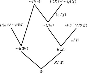
For example, suppose we want to prove the theorem, P(a), from the set of ![]() . First we consider
. First we consider

which is already a set of clauses. From this L, we take two clauses, for example, P(X) V ∨ ∼Q(X) and ∼P(a). If we unify these two clauses using the unification algorithm, we obtain ξ{a/X} as the mgu. If we then apply ξ to P(X) V ∼Q(X) and ∼P(a) we obtain
Now, applying the inference rule of resolution to this, we obtain ∼Q(a) as a resolvent. We then add ∼Q(a) to L.
Next, if we select ∼Q(a) and Q(Y) ∨ R(Z), we obtain ξ = {a/Y} as the mgu using unification. Applying ξ to the two clauses generates
as the set of unified clauses. If we apply the inference rule of resolution to this, we obtain the resolvent R(Z). So, we add R(Z) to L. Similarly, we obtain, for example, the resolvent ∼R(W) from ∼P(A) and P(a) V ∼R(W). We also add ∼R(W) to L. Finally, if we take R(Z) and ∼R(W) from L and apply the unification algorithm, we obtain ξ = {Z/W} as the mgu. Applying ξ and then the resolution to these two clauses, we obtain the empty clause.
In this way we can show the unsatisfiability of a given set of clauses if they are actually unsatisfiable and thus show that w can be proved from W. The process of deleting unsatisfiable clauses using resolution is called a refutation process. The refutation process described in the above example is illustrated in Figure 3.12.
(e) Logical inference and generating representations
The algorithm for theorem proving based on the resolution principle described above can be applied generally to first-order predicate logic, although it usually takes a long time to compute. When a set of clauses is large, the efficiency of computation depends on which clauses we pick for the refutation. On the other hand, by applying this method to the Horn clause logic rather than first-order predicate logic, we can execute efficient theorem proving on a computer. Actually, the basic part of Prolog can be regarded as a language for processing a unification algorithm applied only to Horn clause logic.
We now show how the algorithm for theorem proving based on resolution can be applied to generation and transformation of representations.
First, notice that this algorithm not only determines whether a theorem can be proved or not but also constructs a proof. In other words, the refutation process described above is itself a proof process. So, just as in the case of search described in Section 3.6, we can regard the algorithm as generating a procedure for deriving a formula (theorem) from a set of formulas (an axiom set).
Second, although the proof process is for proving a given theorem, we can generate a new representation by generalizing the process itself, for example, by substituting new variable symbols for some constant symbols. Actually, such a method of generation has been applied to learning by a computer and is called “explanation-based learning.” We will describe this in detail in Chapter 8.
Third, it is known that we can use the unification algorithm for judging the similarity between two sets of well-formed formulas in Horn clause logic. A judgment of similarity is the basis for learning by analogy, which will also be described in Chapter 8.
Thus, theorem proving as logical inference using predicate logic representation is a powerful method for generating representations.
3.8 Production Systems
Production rules as described in Section 2.1 are not usable if we simply describe rules. We need a system for interpreting and executing rules. Such a system is generally called a production system. Like search and logical inference, a production system can be a powerful tool for generating and transforming representations. In this section we explain production systems.
(a) Production systems using ordered rules
First, let us consider the following collection of rules:
where $x, $y, $z axe variables.
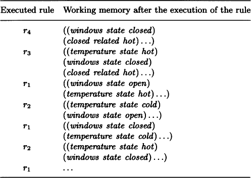
We now define working memory for rules r1-r4. Working memory is represented by a list of lists. Suppose its initial state is
We also suppose that *add and * delete in the action side of the rules are procedures for deleting its argument from working memory and for adding its argument to the top of working memory, respectively.
We examine r1-r4 from the top and execute the action side of a rule whose condition side matches working memory when some constant is substituted for a variable in the rule. By repeating this recognition-action cycle (or recognize-act cycle), working memory changes as shown in Table 3.1 every time a rule is executed.
If we define a rule with an appropriate termination procedure on its action side, we can terminate the execution of the recognition-action cycle, although this is not included in the above example.
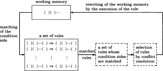
The mechanism of a production system can be summarized as illustrated in the diagram in Figure 3.13. That is, it checks the rules in order from the first one, matching working memory against the condition side of the rule and executing the procedures given in the action side of the rule. If working memory changes because of this, another rule may match. By giving a set of rules and an initial state of working memory to such a system, we can do the inference as exemplified in Table 3.1.
(b) Production systems using a discrimination tree
The above example assigns an order to rules and checks them in order. However, as the number of rules increases, matching takes too long to be practical for computation. To avoid it, we can put the condition sides of rules together and compile them into the form of a discrimination tree.
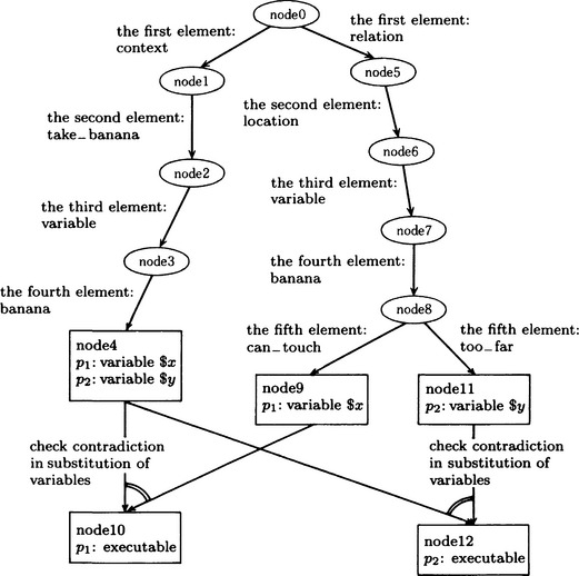
For example, for the following two rules, p1, p2, we can generate the discrimination tree shown in Figure 3.14 before we apply the rules:
We can easily check whether a rule matches the working memory by putting the list in the working memory through the discrimination tree and then checking for a contradiction due to binding variables to constants. Moreover, by remembering states of variable bindings that occurred in the discrimination tree, we can find the set of matched rules by discriminating only lists added or deleted in the previous recognition-action cycle.
However, a system using a discrimination tree may get more than one rule that matches working memory. In such a case, we need to decide which rule to execute. Such a decision is called conflict resolution. The mechanism of a production system that includes conflict resolution will contain the part with broken lines in Figure 3.13.
(c) Production system and generating representations
In a production system, many methods besides those described above can be used. Currently, when we say a production system, we often mean a general framework of an inference system using production rules as a representation. Here we would like to point out that the production systems described in (a) and (b) are suitable for generating rule representation. Suppose we add the following rule to the top of the set of rules, r1−r4:
*build is a procedure for adding to the top of the set of rules a rule that has a name as its first argument and the body of a rule as its second argument.
If we repeat the recognition-action cycle for rules ro−r4 using the method described in (a), ro will be executed after ro is executed twice. As a result, by the procedure in its action side, it will *build the new rule
and add it to the top of the set of rules. When that happens, the new rule rs will be executed next and the inference will proceed differently. This simple example is only for explanation, but we can create complicated changes in the inference process by including variables in the argument of *build, or not writing a whole rule within *build but making it possible to generate parts of the rule by recognition-action cycles. However, in the case of a system using discrimination trees as described in (b), we need to create a new discrimination tree every time a new rule is generated, and as a result the computation will take extra time.
A production system that can generate a new rule by itself during the inference process is called an adaptive production system. We will say more about this kind of system in Chapter 7. In a production system, we do inference by changing working memory. So, if working memory or a part of it represents some object, we can consider it to be a system for generating new representations even if it is not an adaptive production system.
3.9 Inference Using Frames
Like production rules, a system for doing inference is important for semantic networks and frames. We can do such inference by making use of the search techniques described in Section 3.6. In this section, we will consider inference using frames.
In a representation using frames (or semantic networks), nodes are classified as either a class or an instance. A class is used to represent a general object or a class of individual objects, and an instance is used in representing an individual object in a class. For example, when a class called “computer” represents computers as a whole, one particular computer is represented as an instance. On the other hand, as we said in Section 2.11, we can make a set of classes represent a hierarchical structure by adding edges having the slot isa : as a label. In such a structure, if a subclass inherits properties of the superclass, we call it property inheritance. When there is more than one superclass to inherit properties from, we call it multiple inheritance.
In a class hierarchy with inheritance, a complicated problem can arise when properties to be inherited are contradictory. For example, a penguin is a bird but cannot fly. Thus it should not inherit the property “can fly” of a bird. This is because the class called penguin does not satisfy one of the properties, “mobility,” of the class bird. The simplest way to allow exceptions is to describe the property “cannot fly” explicitly as the filler of the slot “mobility” of a penguin, and, if the filler of the slot of a superclass (bird, in this example) is different from the filler of the same slot of the subclass (penguin, in this example), not to inherit the property and give priority to the filler of the subclass. This method is called blocking inheritance.
There have been attempts to represent a frame in first-order predicate logic. For example, “a human being is a mammal” can be represented in a frame: “human being” is a subclass of “mammal” and the filler of the slot isa : of “human being” is “mammal.” This can be expressed by a well-formed formula as
where person and mammal are predicate symbols representing a human being and a mammal, respectively.
We will not explain further the relation between frames and predicate logic in this book. It is important to study the properties of first-order predicates that represent exceptions in frame systems. For example, non-monotonic logic, which will be described in Chapter 8, is useful for formulating the logical meaning of exceptions.
Implementing inheritance on a computer, without multiple inheritance, is easy. However, it may be slow if we compute inheritance dynamically as part of the inference process. Therefore, it may be more effective for the overall performance of an inference system to compute all properties to be inherited by each class and instance before execution. Such a precompiler will decrease the amount of computation necessary during execution, although it will increase the amount of information we need to store. This suggests that, in practical situations, inheritance is not a basic function of inference, but rather it makes programs easier to code and understand.
3.10 Constraint Representation and Relaxation
Some methods of representing an object use the idea of constraint
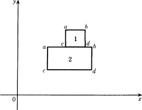
For example, consider the spatial relation on. Suppose there are two rectangles, 1 and 2, in two-dimensional Euclidean space as shown in Figure 3.15. The relation on meaning that 1 “is on” 2 can be represented by the following set of linear simultaneous inequalities:
where xin and yinyin are the x and y coordinates of vertex n of rectangle i, respectively.
We can use this kind of representation not only for metric representations such as coordinate representations but also for symbolic representations such as predicate logic. Generally, the representation of objects by a set of constraints that those objects need to satisfy is called constraint representation. The relaxation method, an algorithm for finding a point that satisfies all the given constraints, is well known as a popular inference method for constraint representation. We will describe the relaxation method in Chapters 5 and 10.
3.11 Summary
In this chapter we explained basic methods for transforming information in a computer from one representation to another and methods for generating new information from old.
3.1. The generalization and transformation of representations are defined as procedures for transforming input information in some representation to output information in another representation.
3.2. Methods of generalization/transformation for pattern functions include convolution integrals, Fourier transforms, sampling, quantization, and transformation to some form of spatial structure representation such as spline function approximation.
3.3. Methods of generalization/transformation for symbolic representations include generation of trees and problem solving based on tree search and state transition.
3.4. Methods of generalization/transformation for more complicated symbolic representations include inference techniques using production systems, frames, and so on, and the relaxation method for constraints.
Exercises
3.1. In (3.8) and (3.9) in Section 3.2(b), show that we can obtain (3.10) and (3.11) if we do the appropriate variable transformation and extend it to two dimensions.
3.2. The following expression is called the Laplacian of the function f{x, y):
Prove that
3.3. Suppose a function f(x) is defined as
Find the values of x and y that make f(x) the smallest. (Hint: use the Lagrange multiplier method given in Section 4.5.)
3.4. A weighted directed tree is a directed tree with a weight on every edge. Given a weighted directed graph, G = (V, E, W), write an algorithm for finding a subtree of G such that the sum of its weights is the smallest. (Such a tree is called a minimum spanning tree of the original graph G.) For simplicity, we assume that G is a connected graph and does not include an edge of the form (v, v) (i.e., a self-loop).
“If something is an LSI chip, then it can be used in the computer called bonyson.”
“A VLSI chip that can be used in a computer can be used in the CPU of that computer.” “m68386 is a VLSI chip.”
Given the above information, determine which computer can use m68386 for CPUs. Use a theorem-proving algorithm based on the resolution principle.
3.6. Suppose the discrimination tree shown in Figure 3.14 is generated for the production rules p1 and p2 shown in Section 3.8(b) and its working memory looks like the following:
Explain how the recognition-action cycle will be executed.
3.7. Suppose the slot “walking method” and its filler “walks on two legs” axe given in the frame for a “human being.” Represent the relation between these three using predicate logic. Also, explain, using examples, the difference between inference using frames and inference in predicate logic.