![]()
Designing Numerical Classes
At the heart of any high-performance financial application there is a set of well-designed numerical classes. These classes are responsible for the implementation of concepts that are an integral part of tasks such as financial modeling, forecasting, and analysis of investment decisions. Without the support of mathematical models, it would be very difficult to propose and evaluate effective investment methodologies. That is why, as a programmer in the financial industry, you need to familiarize yourself with the best strategies to design and implement mathematically oriented code in C++. Although it is not necessary to become a math expert to use these programming techniques, it helps to possess a basic understanding of the most important numerical issues that need to be dealt with in your financial programming assignments.
This chapter will show you how to create classes that can run efficiently when used in numerically oriented, production-ready code. You will also see recipes that show how to integrate existing numerical classes and algorithms into your applications.
Some of the concepts discussed in the code examples in this chapter include the following:
- How to design and implement an efficient matrix class.
- How to supporting common matrix operations.
- How to perform calculations at compilation time.
- How to calculate factorial numbers using templates.
- How to represent ratios as data types.
- How to use and generate stochastic values using the boost library.
Representing Matrices in C++
Implement a class that represents a matrix with some common associated operations, such as addition, subtraction, transposition, and multiplication.
Solution
Matrix manipulation is one of the basic operations in numerical computing. C++ doesn’t have a matrix type, however, and it becomes necessary to implement matrices in most financial projects. The good news is that it is relatively easy to use algorithms already present in the standard templates library (STL) for this purpose, as you will see in the following coding recipe.
A matrix is just a two-dimensional arrangement of numbers, with which one can perform a set of standard mathematical transformations. In terms of data organization in memory, a matrix is not very different from a vector. Considering this similarity, we can take advantage of existing vector operations to facilitate the implementation of a Matrix class. Here is a possible definition for such a class.
class Matrix {
public:
    typedef std::vector<double> Row;

    Matrix(int size, int size2);
    Matrix(int size);
    Matrix(const Matrix &s);
    ~Matrix();
    Matrix &operator=(const Matrix &s);

    void transpose();
    double trace();
    void add(const Matrix &s);
    void subtract(const Matrix &s);
    void multiply(const Matrix &s);

    Row & operator[](int pos);
private:
    std::vector<Row> m_rows;
};
Notice that, at the beginning of the public interface of the class, I used a public typedef to define a Row type. Since a row is just a vector of numbers, I want to avoid typing something as involved as std::vector<std::vector< > > to talk about simple rows. This is also a good measure that can help you avoid mistakes when defining new variables and member functions. As a result of this typedef, all the data stored in the matrix is declared as a vector of Row objects in the private section of the Matrix class.
The simple Matrix class just presented has two constructors.
Matrix(int size);
Matrix(int m, int n);
The first one creates a square matrix, that is, a matrix with the same number of rows and columns. The second constructor is used to create a more generic rectangular matrix, with m rows and n columns.
To make the matrix operate more like its counterpart, the vector, you can introduce a subscript operator to act as an access helper. In this way, it is possible to set and retrieve the value of specific entries in the matrix using native syntax. The implementation of the operator is straightforward, then, since we can refer to each individual row in the matrix.
Matrix::Row &Matrix::operator[](int pos)
{
    return m_rows[pos];
}
Next, we consider some elementary operations on matrices. The first operation is transposition, which is defined as the exchange of elements between rows and columns. That is, if A is a matrix, we need to interchange values between A[i][j] and A[j][i].
The second common operation on matrices is calculating the trace, which is defined as the sum of the elements in the main diagonal (that is, those elements with the same row and column position). This can be implemented as follows:
double Matrix::trace()
{
    if (m_rows.size() != m_rows[0].size())
    {
        return 0;
    }
    double total = 0;
    for (unsigned i=0; i<m_rows.size(); ++i)
    {
        total += m_rows[i][i];
    }
    return total;
}
The first if statement checks if the matrix has a different number of rows and columns, in which case the trace operation is not defined. The for statement then iterates over the diagonal, adding those values to the total variable, which is returned at the end of the member function.
The Matrix class also implements the operations of adding and subtracting matrices. To add one matrix to another, you just need to add the individual elements of the first one to the corresponding elements in the second matrix. Similarly, the subtraction of matrices is defined element-wise. These operations are straightforward to implement in C++.
Finally, you can see how to implement matrix multiplication. In this case, you need to compute a new matrix, where each element is determined as the sum of the products of the i-th row and j-th column. The resulting matrix has dimensions determined by the number of rows in the current matrix and number of columns in the parameter matrix. The main part of the algorithm is the following:
std::vector<Row> rows;
for (unsigned i=0; i<m_rows.size(); ++i)
{
    std::vector<double> row;
    for (unsigned j=0; j<s.m_rows.size(); ++j)
    {
        double Mij = 0;
        for (unsigned k=0; k<m_rows[0].size(); ++k)
        {
            Mij += m_rows[i][k] * s.m_rows[k][j];
        }
        row.push_back(Mij);
    }
    rows.push_back(row);
}
m_rows.swap(rows);
In this code, we have three loops that range over the different dimensions of the original and the parameter matrix. The value Mij represents the element in position [i][j] for the resulting matrix. Notice that to simplify storage management, the algorithm performs the assignments in a new set of rows. Then, the results are stored in place of the existing values in the last line, using the swap function.
After the Matrix class has been defined, I have also added a few free operators that make it easier to work with the previously defined operations. These operators make sure that you can add, subtract, and multiply matrices using a syntax similar to that of native operations, although assuming a slight overhead for the temporary objects that become necessary. Here, for example, is the definition of operator *.
Matrix operator*(const Matrix &s1, const Matrix &s2)
{
        Matrix s(s1);
        s.multiply(s2);
        return s;
}
Complete Code
The ideas just described have been implemented in the Matrix class, presented here in Listing 5-1. This is a class that I will use in other examples in the next chapters of this book, so you should be familiar with its definition and main uses.
Listing 5-1. The Matrix Class
//
//  Matrix.h

#ifndef __FinancialSamples__Matrix__
#define __FinancialSamples__Matrix__

#include <vector>

class Matrix {
public:
    typedef std::vector<double> Row;

    Matrix(int size, int size2);
    Matrix(int size);
    Matrix(const Matrix &s);
    ~Matrix();
    Matrix &operator=(const Matrix &s);

    void transpose();
    double trace();
    void add(const Matrix &s);
    void subtract(const Matrix &s);
    void multiply(const Matrix &s);

    Row & operator[](int pos);
private:
    std::vector<Row> m_rows;
};

// free operators
//
Matrix operator+(const Matrix &s1, const Matrix &s2);
Matrix operator-(const Matrix &s1, const Matrix &s2);
Matrix operator*(const Matrix &s1, const Matrix &s2);

#endif /* defined(__FinancialSamples__Matrix__) */

//
//  Matrix.cpp

#include "Matrix.h"

Matrix::Matrix(int size)
{
    for (unsigned i=0; i<size; ++i )
    {
        std::vector<double> row(size, 0);
        m_rows.push_back(row);
    }
}

Matrix::Matrix(int size, int size2)
{
    for (unsigned i=0; i<size; ++i )
    {
        std::vector<double> row(size2, 0);
        m_rows.push_back(row);
    }
}

Matrix::Matrix(const Matrix &s)
: m_rows(s.m_rows)
{
}

Matrix::~Matrix()
{
}

Matrix &Matrix::operator=(const Matrix &s)
{
    if (this != &s)
    {
        m_rows = s.m_rows;
    }
    return *this;
}

Matrix::Row &Matrix::operator[](int pos)
{
    return m_rows[pos];
}

void Matrix::transpose()
{
    std::vector<Row> rows;
    for (unsigned i=0;i <m_rows[0].size(); ++i)
    {
        std::vector<double> row;
        for (unsigned j=0; j<m_rows.size(); ++j)
        {
            row[j] = m_rows[j][i];
        }
        rows.push_back(row);
    }
    m_rows.swap(rows);
}

double Matrix::trace()
{
    if (m_rows.size() != m_rows[0].size())
    {
        return 0;
    }
    double total = 0;
    for (unsigned i=0; i<m_rows.size(); ++i)
    {
        total += m_rows[i][i];
    }
    return total;
}

void Matrix::add(const Matrix &s)
{
    if (m_rows.size() != s.m_rows.size() ||
        m_rows[0].size() != s.m_rows[0].size())
    {
        throw new std::runtime_error("invalid matrix dimensions");
    }
    for (unsigned i=0; i<m_rows.size(); ++i)
    {
        for (unsigned j=0; j<m_rows[0].size(); ++j)
        {
            m_rows[i][j] += s.m_rows[i][j];
        }
    }
}

void Matrix::subtract(const Matrix &s)
{
    if (m_rows.size() != s.m_rows.size() ||
        m_rows[0].size() != s.m_rows[0].size())
    {
        throw new std::runtime_error("invalid matrix dimensions");
    }
    for (unsigned i=0; i<m_rows.size(); ++i)
    {
        for (unsigned j=0; j<m_rows[0].size(); ++j)
        {
            m_rows[i][j] += s.m_rows[i][j];
        }
    }
}

void Matrix::multiply(const Matrix &s)
{
    if (m_rows[0].size() != s.m_rows.size())
    {
        throw new std::runtime_error("invalid matrix dimensions");
    }
    std::vector<Row> rows;
    for (unsigned i=0; i<m_rows.size(); ++i)
    {
        std::vector<double> row;
        for (unsigned j=0; j<s.m_rows.size(); ++j)
        {
            double Mij = 0;
            for (unsigned k=0; k<m_rows[0].size(); ++k)
            {
                Mij += m_rows[i][k] * s.m_rows[k][j];
            }
            row.push_back(Mij);
        }
        rows.push_back(row);
    }
    m_rows.swap(rows);
}

Matrix operator+(const Matrix &s1, const Matrix &s2)
{
        Matrix s(s1);
        s.subtract(s2);
        return s;
}

Matrix operator-(const Matrix &s1, const Matrix &s2)
{
        Matrix s(s1);
        s.subtract(s2);
        return s;
}

Matrix operator*(const Matrix &s1, const Matrix &s2)
{
        Matrix s(s1);
        s.multiply(s2);
        return s;
}
Using Templates to Calculate Factorials
Create a template-based class that can be used to calculate factorials at compile time.
Solution
Templates provide an easy way to apply the same code across data types, allowing programmers to create generic, reusable code. The best example of this is the STL, with its many containers and associated algorithms. However, templates can also be used to perform numerical tasks due to their ability to receive integer numbers, in addition to data types, as formal arguments. In this coding recipe, you will see how templates can be employed to perform some simple calculations at compilation type.
Template-based computation can be seen as a useful strategy to reduce the runtime overhead of numeric algorithms. After all, if you’re able to perform some of the calculations at compilation time, less time will be necessary to perform the complete computation each time you execute the compiled code.
One of the biggest surprises for people who start working with template-based computing is that calculated values cannot simply be returned as the output of functions. Since functions can return any value at runtime, a traditional function cannot serve as the basis for compile-time calculations. Instead, you need a way to store values inside the class as a constant, which can then become readily available to the compiler. One of the ways to achieve this in C++ is with an enumeration. For example, consider
enum {
   result = 1
};
This fragment defines a constant, integral value that can be later referenced in the program. If a constant expression is used (instead of a number) in the right-hand side of the declaration, the result value can be later employed in the program to access the desired value.
The next thing you need is a way to pass numbers as parameters to the class template. In C++, you can declare templates that take as parameters an int value (or one of its several variations such as long and char). The general syntax that can be used to perform calculations as part of a template is the following:
template <int N>
class CompileTime {
public:
  enum {  result = ConstantExpressionDependingOnN };
};
where ConstantExpressionDependingOnN is an expression that in some way depends on the parameter N and can be used to calculate the desired value. You can see that the code in this example will use this general format to perform compile-time calculations.
Once you find a way to execute calculations at compilation time, the next step is to introduce concepts such as iteration to your code. In C++ templates, it is not possible to write loops, such as for or while, as part of a constant expression. All C++ loops are executed at runtime, which makes them unusable for compile-time operations. Thankfully, templates provide a specialization mechanism that can be used to implement recursion, a technique that can be used to achieve the same effects as looping.
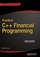
For example, if a template uses a single integer parameter, you can specialize that parameter with a base case alongside a generic version that handles the common case. Together, these cases are enough to simulate a loop that starts with the generic case and terminates the computation once the special case is reached. Figure 5-1 presents an illustration of this mechanism, where the following example is considered:
// general case
template <int N>
class Double {
public:
  enum {  result = 2 + Double<N-1>  };
};

// specialization for the base case
template <>
class Double<1> {
public:
  enum {  result = 2 };
};
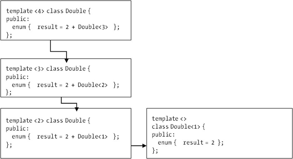
Figure 5-1. An example of computation using template specialization. The general case is instantiated with the integer 4, and new instantiations are used until the specialization for Double<1> is reached
This shows how you can compute the double of an integer number using template-based recursion. The general case is stated at the top, where the result value is defined as the expression 2 + Double<N-1>.
To find the value of that expression, the compiler will need to expand it inline, decreasing the value of N each time and calling Double with the new value. The second part of the declaration allows this process to end, introducing a base value. The declaration reads
template <>
class Double<1>
This tells the compiler that Double<1> is a specialization of a generic template, for the particular value of 1. Therefore, when the template Double is applied to 1, the result calculated will be the value 2, as desired.
A similar strategy can be used to solve multiple problems, including the required task of computing factorials. The first part is to define the general case, which contains a recurring expression.
template <long N>
class Factorial {
public:
    enum {
        result = Factorial<N-1>::result * N
    };

};
The second part of the solution is the base case, which will determine the value of Factorial<0>. This can be written as
template <>
class Factorial<0> {
public:
    enum {
        result = 1
    };
};
We can test the preceding code with a few calls to the Factorial template. The example is included as part of the showFactorial function.
void showFactorial()
{
    std::cout << " Some factorial values: " << std::endl;
    std::cout << "fact(5)= " << Factorial<5>::result;
    std::cout << "fact(7)= " << Factorial<7>::result;
    std::cout << "fact(9)= " << Factorial<9>::result;
}
Finally, you can also use the Factorial class as the basis of other compile-time computations. For example, here is how you can use Factorial to calculate the choice number (the number of combinations of N objects, taken in groups of P).
template <int N, int P>
class ChoiceNumber {
public:
    enum {
        result = Factorial<N>::result / (Factorial<P>::result * Factorial<N-P>::result)
    };
};
Notice that here you don’t need a base case, since there is actually no recursion involved. The ChoiceNumber class template is just using Factorial directly to perform the compile-time calculation as its result.
The nice thing about compile-time computations using templates is that you can use the same strategy discussed here to compute very different functions. As long as you can represent the computation as a recursion, the scheme described previously can be employed with little modification. In this way, you will be using the power of the compiler to perform calculations ahead of time, and possibly saving a lot of time later, when the program is actually running.
![]() Caution While the ability of calculating values using templates is very useful, you may want to avoid using them frequently, since they may slow down compilation. Long compilation times may be the biggest adverse effect of overreliance on templates. Ideally, you should consider the trade-off between compilation time and runtime savings before deciding if a computation should be performed using templates at compilation time instead of runtime.
Caution While the ability of calculating values using templates is very useful, you may want to avoid using them frequently, since they may slow down compilation. Long compilation times may be the biggest adverse effect of overreliance on templates. Ideally, you should consider the trade-off between compilation time and runtime savings before deciding if a computation should be performed using templates at compilation time instead of runtime.
Complete Code
Here you have an example of using templates to calculate factorials at compile time. The important part of the implementation is in the header file (FactorialTemplate.h) shown in Listing 5-2. This is necessary, since templates need to be visible to the client at the moment they are used. The cpp file shows some sample uses of the template.
Listing 5-2. The FactorialTemplate.h Header File
//
//  FactorialTemplate.h

#ifndef __FinancialSamples__FactorialTemplate__
#define __FinancialSamples__FactorialTemplate__

template <long N>
class Factorial {
public:
    enum {
        result = Factorial<N-1>::result * N
    };
private:

};

template <>
class Factorial<0> {
public:
    enum {
        result = 1
    };
};

template <int N, int P>
class ChoiceNumber {
public:
    enum {
        result = Factorial<N>::result / (Factorial<P>::result * Factorial<N-P>::result)
    };
};

void showFactorial();

#endif /* defined(__FinancialSamples__FactorialTemplate__) */

//
//  FactorialTemplate.cpp

#include "FactorialTemplate.h"

#include <iostream>

void showFactorial()
{
    std::cout << " Some factorial values: " << std::endl;
    std::cout << "fact(5)= " << Factorial<5>::result;
    std::cout << "fact(7)= " << Factorial<7>::result;
    std::cout << "fact(9)= " << Factorial<9>::result;
}

int main(int argc, const char **argv)
{
    std::cout << "factorial(6) = " << Factorial<6>::result;
    std::cout << "
 choiceNumber(5,6) = " <<  << ChoiceNumber<6,2>::result;
    showFactorial();
    return 0;
}
Running the Code
You can compile and run the FactorialTemplate class to test the concepts you have just learned. For that purpose, you can use the gcc compiler, which can generate an application using the following command:
gcc -o factorial FactorialTemplate.cpp
After a few seconds, the binary file factorial will be created with the desired functionality. You can run the program by just calling it from the command line
./factorial
You can also click the executable if running on a Windows machine. This would result in the following output:
factorial(6)= 720
choiceNumber(5,6) = 15
factorial(5)= 120
factorial(7)= 5040
factorial(9)= 362880
Representing Calmar Ratios at Compile Time
The Calmar ratio is a measure of investment returns as compared to possible annual losses. It is used to compare investments with different risk profiles. The Calmar ratio is defined as the average annual rate of return for a given period, divided by the maximum drawdown (i.e., the maximum loss) during the same period. If you consider the same rate of return, investments with higher Calmer ratio had lower risk during the considered period. Create C++ code to represent Calmar ratios using compile-time techniques.
Solution
When writing numerical algorithms, it is frequently useful to represent certain quantities as constants. Some of these mathematical constants, however, are better denoted as ratios. For example, physical quantities frequently employ units of measurement, which are regularly represented as the ratio of other more fundamental units. As a consequence, ratios are a specific type of mathematical constant that can benefit from a more specific, high-level representation.
In this coding example, you will solve this problem using a simple library that is part of the boost repository. The library is called ratio and uses templates to represent mathematical quantities such as the standard Calmar ratio of an investment. The used representation can also be checked during compilation.
The basic template provided in the ratio library is simply called ratio. Its operation requires two template parameters, respectively, the numerator and the denominator. These parameters can either be simple numeric types, such as int, or other types previously declared using the ratio template. Types defined with the ratio template for different inputs are fundamentally different, and the compiler will enforce the correctness of any arithmetic operations involving these values.
One of the main advantages of using the ratio template is that it also provides some common compile-time operations. These operations can be used to perform standard mathematical transformations to the quantities defined with the template. Such operations include
- boost::ratio_add
- boost::ratio_subtract
- boost::ratio_multiply
- boost::ratio_add
- boost::ratio_negate
Using these operations, you can define derived types and constants, which are derivatives of the original ratio types. You can also use a few template-based operations to perform logical comparisons on such ratios, such as
- boost::ratio_equal
- boost::ratio_not_equal
- boost::ratio_less
- boost::ratio_less_equal
- boost::ratio_greater
- boost::ratio_greater_equal
You can start using the ratio library by importing the main header file <boost/ratio.hpp>. Then, you can start defining objects for each desired ratio using boost::ratio.
#include <boost/ratio.hpp>

boost::ratio<1, 2> one_half;
boost::ratio<1, 3> one_third;
boost::ratio<2, 5> two_fifths;
Once a boost::ratio object has been defined, you can retrieve its information at runtime using the num and den member variables, which correspond to the numerator and denominator, respectively. For example,
std::cout << "one_third numerator: " << one_third.num
          << " denominator: " << one_third.den;
Representing Calmar Ratios
With the help of the ratio library it is possible to create a few useful financial types such as a Calmar ratio. The Calmar ratio is defined as the annual rate of return of an investment divided by its maximum drawdown during the known period. Thus, a CalmarRatio type can be defined as follows:
typedef boost::ratio<1, 1>::type CalmarRatioType;
From now on, CalmarRatioType can be used to represent quantities with a numerator and denominator at compile time. More interestingly, suppose that we want to be able to represent Calmar ratios using percentages as well as percentage points (1/100%). The definitions would then become
typedef boost::ratio<1, 100>::type CalmarRatioBPS;
typedef boost::ratio<1, 1>::type CalmarRatioPerc;
With these two types, we could create a template-based class to return information about the particular ratio, such as the maximum drawdown and the performance of the given object. The implementation is as follows:
template <class Ratio>
class CalmarRatio {
public:
        CalmarRatio(double calmar, double ret) : m_calmar(calmar), m_return(ret) {}
        virtual ~CalmarRatio() {}

        double getReturn();
        double getDrawDown()
        {
                return m_return / m_calmar * m_ratio.den;
        }
private:
        Ratio m_ratio;
        double m_calmar;
        double m_return;
};
The class is a template that receives the desired ratio type, either CalmarRatioPerc or CalmarRatioBPS. Of course, other ratio types could be supported if needed. Let’s check the getDrawDown member function. The standard definition uses the den variable to calculate the drawdown of the investment. However, different versions of this member function can be created using template specializations. The following implementation provides an example:
template <>
double CalmarRatio<CalmarRatioBPS>::getDrawDown()
{
        return  m_return / m_calmar * m_ratio.den * 100;
}
In this case, since the template is specialized for the CalmarRatioBPS, the standard drawdown is multiplied by 100. This is necessary because the denominator is expressed in basis points, instead of percentages.
Complete Code
Listing 5-3 presents an implementation for the CalmarRatio class. Notice the use of the boost::ratio template to model different ratio types and how they are used by the main class.
Listing 5-3. The CalmarRatio Class
// CalmarRatio.h
//

#ifndef CALMARRATIO_H_
#define CALMARRATIO_H_

#include <boost/ratio.hpp>

typedef boost::ratio<1, 1>::type CalmarRatioType;
typedef boost::ratio<1, 100>::type CalmarRatioBPS;
typedef boost::ratio<1, 1>::type CalmarRatioPerc;

template <class Ratio>
class CalmarRatio {
public:
        CalmarRatio(double calmar, double ret) : m_calmar(calmar), m_return(ret) {}
        ~CalmarRatio() {}

        double getReturn()
        {
                return m_return;
        }

        double getDrawDown()
        {
                return m_return / m_calmar * m_ratio.den;
        }
private:
        Ratio m_ratio;
        double m_calmar;
        double m_return;
};

template <>
double CalmarRatio<CalmarRatioBPS>::getDrawDown()
{
        return  m_return / m_calmar * m_ratio.den * 100;
}

#endif /* CALMARRATIO_H_ */

// CalmarRatio.cpp
//

#include "CalmarRatio.h"

#include <iostream>

boost::ratio<1, 2> one_half;
boost::ratio<1, 3> one_third;

void createCalmarRatio()
{
        CalmarRatio<CalmarRatioPerc> ratio(0.15, 11);
}

void printRatios()
{
        std::cout << "one_third numerator: " << one_third.num
                  << " denominator: " << one_third.den;
}

int main()
{
        CalmarRatio<CalmarRatioPerc> ratio(0.110, 3.12);
        std::cout << "return: " << ratio.getReturn()
                  << " drawdown: " << ratio.getDrawDown() << std::endl;

        CalmarRatio<CalmarRatioBPS> bpsRatio(480, 2.15);
        std::cout << "return: " << bpsRatio.getReturn()
                  << " drawdown: " << bpsRatio.getDrawDown() << std::endl;

}
Running the Code
We tested the sample application containing the CalmarRatio class and its associated code in a UNIX system using the gcc compiler. You can compile the cpp file presented earlier using a build system such as make, with its related makefile. Or you can just build the application directly with the compiler, using the following command line:
gcc -o calmarRatio CalmarRatio.cpp
The resulting executable file can be called from the terminal. It will display the result of the Calmar ratios in the following way:
return: 3.12 drawdown: 28.3636
return: 2.15 drawdown: 44.7917
As you see, the code treats the parameters differently, with results interpreted according to the type of Calmar ratio used. The first example uses a CalmarRatioPerc, which regards the Calmar ratio as applied to a percentage. The second example uses a CalmarRatioBPS representation, which works with basis points instead of percentages. The results, however, are displayed correctly according to their respective return and drawdown.
Generating Statistical Data
Create data using statistical distributions such as Gaussian (normal distribution) and chi-squared.
Solution
When working with trading algorithms, it is frequently useful to test the operation of such strategies on artificially generated prices. If we consider that most of the short-term movements of the market have a stochastic component, we can use random number generators to approximate the values of typical price-related time series.
In this section, we investigate how to generate statistically based data that can later be used to test trading strategies. To do this, you can use one of the many libraries currently available for the generation of statistical values in C++. These libraries operate similarly to random number generators, with a few differences. Traditional random number generators are used to produce random integer values. Such numbers can be, with some work, converted into uniformly distributed random numbers in a given interval, such as between 0 and 1.
For more advanced uses, however, it is interesting to generate random numbers from a particular probability distribution. Such probability distributions are based on standard random processes and include the Gaussian distribution (also known as normal distribution) and the Chi-squared distribution (a form of skewed normal distribution). See Figure 5-2. These distributions can be used to generate stochastic numbers that are more representative of the stock market.
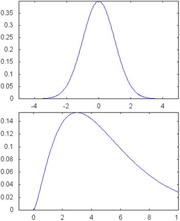
Figure 5-2. Plots for two probability distribution functions (PDF) available in the boost::math namespace. The top plot is for a normal distribution with parameters 0 and 1. The bottom plot is for the chi-squared distribution with parameter 5
In this recipe, I will show you how to use the boost::math namespace, where you declare a set of objects representing statistical distributions. The use of a library for this task makes it possible to concentrate on the design of your algorithm, instead of having to re-implement such a common statistic utility function, which has already been made available in many programming libraries. I also use the boost::random library to generate random data points based on these distributions.
Probability Distributions
Before I start, let me give you a quick overview of probability distributions and their uses. Probability distributions are a mathematical representation of parameterized random processes that frequently occur in nature. For example, the most basic probability distribution is the uniform distribution, in which points occur with the same probability over the whole interval in which the function is defined. Thus, each time a new event occurs according to this distribution (assuming that it has been defined for numbers between 1 and 2), its value may be any real number between 1 and 2 with equal probability. The uniform distribution has an important role because values generated under uniform random probability can be converted into other probability distributions.
Another important distribution is normal (or Gaussian) distribution. The normal distribution has two parameters: the mean (average) value and the standard deviation. Normally distributed random events occur with highest probability around the mean, and the probability of an event occurring further away decreases quickly. The resulting probability distribution is bell-shaped to indicate this characteristic of the probability space. It has been observed that many natural phenomena follow the normal distribution, especially when large numbers of observations are considered. Figure 5-2(top) shows a plot of the probability distribution function (PDF) for a normal (also known as Gaussian) random variable.
Other probability distributions are also used in financial applications. You can see a quick list of the most important in Table 5-1. Each distribution has a common usage pattern and associated parameters that can be used to describe the range of probabilities as well as the shape of the resulting function.
Table 5-1. A Few Commonly Used Distributions with Their Parameters and Corresponding boost::math Identifier
|
Distribution |
Parameter(s) |
boost::math identifier |
|---|---|---|
|
Bernoulli |
Probability of success |
boost::math::bernoulli_distribution |
|
Beta |
Alpha and Beta (real values) |
boost::math::beta_distribution |
|
Binomial |
Number of trials and success probability |
boost::math:: binomial_distribution |
|
Cauchy |
Location and scale |
boost::math::cauchy_distribution |
|
Chi-squared |
Degrees of freedom |
boost::math::chi_squared_distribution |
|
Exponential |
Lambda (rate) |
boost::math::exponential_distribution |
|
Geometric |
Success probability |
boost::math::geometric_distribution |
|
Hypergeometric |
N, K, and number of trials |
boost::math::hypergeometric_distribution |
|
Log-normal |
Mean and sigma |
boost::math::lognormal_distribution |
|
Logistic |
Mean and scale |
boost::math::logistic_distribution |
|
Normal (Gaussian) |
Mean and sigma |
boost::math::normal_distribution |
|
Poisson |
Lambda (rate) |
boost::math::poisson_distribution |
|
Student’s t-Distribution |
Degrees of freedom (real value) |
boost::math::students_t_distribution |
|
Triangular |
Extremes and middle point |
boost::math::triangular_distribution |
|
Uniform |
Start and end of interval |
boost::math::uniform_distribution |
In order to use some of these probability distributions in your code, you can include the header file <boost/math/distributions.hpp>. First, you need to make sure that boost is properly installed in your system (check the installation instructions on the www.boost.org web site). The last column of Table 5-1 lists the distribution names.
Once you import a particular distribution, you can use it to respond to common questions such as the following: What is the mean of the distribution? What is the respective quantile for a particular value? What is the CDF of a particular value? You will see some of these questions being answered in class DistributionData, which is listed here.
Another responsibility of class DistributionData is to generate random numbers for some distributions, given the required parameters. A distribution-specific random number is created when the distribution object is called. You need to pass a uniform random number generator, which is also provided by boost. You can store these values in a vector, and return them at the end of the member function. Here is an example of how this process works for Gaussian-distributed data.
std::vector<double> DistributionData::gaussianData(int nPoints, double mean, double sigma)
{
        std::vector<double> data;

        boost::random::normal_distribution<> distrib(mean, sigma);

        for (int i=0; i<nPoints; ++i)
        {
                double val = distrib(random_generator);
                data.push_back(val);
        }

        return data;
}
Two other common probability distributions are the gamma and log-normal distributions. The gamma distribution can be interpreted as a generalized version of the normal distribution, in which you can control the shape and scale of the probabilities. Figure 5-3 (top) shows an example of the gamma distribution. The log-normal distribution is another possible generalization of the normal distribution, and it can be interpreted as the product of several positive and independent random variables. Its PDF is presented in Figure 5-3 (bottom). The log-normal distribution is included as one of the distributions supported by class DistributionData.
Figure 5-3. Plots for two probability distribution functions (PDF) available in the boost::math namespace. The top plot is for a gamma distribution with parameters 1 and 2. The bottom PDF is for the log-normal distribution with parameters 0 and 1
Complete Code
In Listing 5-4, I show the implementation for a class that generates data using a few of the probability distributions available in the boost::random template library. The main class is called DistributionData, and you can use it to generate numbers, as well as calculate quantiles for some distributions.
Listing 5-4. The DistributionData Class
// DistributionData.h
//

#ifndef DISTRIBUTIONDATA_H_
#define DISTRIBUTIONDATA_H_

#include <vector>

// class responsible for generating data basic on common probability distributions
//
class DistributionData {
public:
        // standard constructor and destructor
        DistributionData();
        ~DistributionData();

        // random data generation based on the given parameters.
        // each function returns a vector with nPoints random values.
        std::vector<double> gaussianData(int nPoints, double mean, double sigma);
        std::vector<double> exponentialData(int nPoints, double rate);
        std::vector<double> chiSquaredData(int nPoints, int degreesOfFreedom);
        std::vector<double> logNormalData(int nPoints, double mean, double sigma);

        // returns the quantile of the give value x, corresponding to the parameters provided.
        //
        double gaussianQuantile(double x, double mean, double sigma);
        double chiSquaredQuantile(double x, int degreesOfFreedom);
        double exponentialQuantile(double x, double rate);
        double logNormalQuantile(double x, double mean, double sigma);
};

#endif /* DISTRIBUTIONDATA_H_ */

// DistributionData.cpp
//

#include "DistributionData.h"

#include <boost/math/distributions.hpp>

using boost::math::quantile;

#include <boost/random.hpp>
#include <boost/random/normal_distribution.hpp>

static boost::rand48 random_generator;

DistributionData::DistributionData()
{
}

DistributionData::~DistributionData()
{
}

std::vector<double> DistributionData::gaussianData(int nPoints, double mean, double sigma)
{
        std::vector<double> data;

        boost::random::normal_distribution<> distrib(mean, sigma);

        for (int i=0; i<nPoints; ++i)
        {
                double val = distrib(random_generator);
                data.push_back(val);
        }

        return data;
}

std::vector<double> DistributionData::exponentialData(int nPoints, double rate)
{
    std::vector<double> data;

        boost::random::exponential_distribution<> distrib(rate);

        for (int i=0; i<nPoints; ++i)
        {
                double val = distrib(random_generator);
                data.push_back(val);
        }

        return data;
}

std::vector<double> DistributionData::logNormalData(int nPoints, double mean, double sigma)
{
    std::vector<double> data;

        boost::random::lognormal_distribution<> distrib(mean, sigma);

        for (int i=0; i<nPoints; ++i)
        {
                double val = distrib(random_generator);
                data.push_back(val);
        }

        return data;
}

std::vector<double> DistributionData::chiSquaredData(int nPoints, int degreesOfFreedom)
{
        std::vector<double> data;

        boost::random::chi_squared_distribution<> distrib(degreesOfFreedom);

        for (int i=0; i<nPoints; ++i)
        {
                double val = distrib(random_generator);
                data.push_back(val);
        }

        return data;
}

double DistributionData::gaussianQuantile(double x, double mean, double sigma)
{
        boost::math::normal_distribution<> dist(mean, sigma);

        return quantile(dist, x);
}

double DistributionData::chiSquaredQuantile(double x, int degreesOfFreedom)
{
        boost::math::chi_squared_distribution<> dist(degreesOfFreedom);

        return quantile(dist, x);
}

double DistributionData::exponentialQuantile(double x, double rate)
{
    boost::math::exponential_distribution<> dist(rate);

        return quantile(dist, x);
}

double DistributionData::logNormalQuantile(double x, double mean, double sigma)
{
    boost::math::lognormal_distribution<> dist(mean, sigma);

        return quantile(dist, x);
}

namespace  {
    template <class T>
    void printData(const string &label, const T &data)
    {
        cout << " " << label << ":  ";
        for (auto i : data)
        {
            cout << i << " ";
        }
        cout << endl;
    }
}

int main()
{
    DistributionData dData;
    auto gdata = dData.gaussianData(10, 5, 2);
    printData("gaussian data", gdata);

    auto edata = dData.exponentialData(10, 4);
    printData("exponential data", edata);

    auto kdata = dData.chiSquaredData(10, 5);
    printData("chi squared data", kdata);

    auto ldata = dData.logNormalData(10, 8, 2);
    printData("log normal data", ldata);
    return 0;
}
Running the Code
You can compile the code in Listing 5-4 using any standard-compliant C++ compiler. You need to have boost installed in your system, as discussed in the previous sections. Following is an example of the expected output (exact numbers will vary depending on your particular implementation and random numbers used):
./distributionData
gaussian data:  7.12699 5.56941 5.91951 3.44111 4.89098 4.95243 7.33077 10.6359 5.00597 3.08975
exponential data:  0.108161 0.212945 0.0355506 0.0165794 0.753239 0.041679 0.219658 0.0610242 0.410622 0.0378433
chi squared data:  6.12073 2.14098 1.57523 6.49539 3.15154 1.47554 8.39545 9.07183 2.77768 5.05356
log-normal data:  1573.09 473.919 370.7 1212.54 1530.16 323705 2586.73 35919.6 628.913 372.41
Conclusion
Numerical classes and functions play a very important role in the development of financial engineering models. They offer the basic level of mathematical support needed for the creation of sophisticated trading strategies. In this chapter, you explored some of the most common numerical libraries.
First, I discussed algorithms based on matrix computation, and how they can be represented using STL-based containers. The STL also provides a wealth of algorithms, which can be used in numerical applications as well as in other generic programming tasks. Next, you learned how to use the compile-time facilities provided by the C++ template mechanism. You have seen examples of how to employ such template-based facilities to calculate the factorial of a number. The same concepts can be extended for many other uses as well. You have also learned about the use of ratio templates, and how they can represent financial concepts such as the Calmar ratio.
Probability distributions are another area of numerical algorithms that have a strong presence in financial applications. The testing of investment strategies usually involves the generation of stochastic data, as a way of simulating possible economic scenarios. You learned how to generate random values based on some of the most common probability distributions. Such distributions are provided by a few numeric libraries, and in this chapter I have used boost::math and boost::random for this purpose. Together, these libraries provide a way to generate random data, as well as returning relevant information about specific distributions such as mean, standard deviation, quantiles, and other related attributes.
Data visualization is another area of programming that is very important in the development of effective financial algorithms. In the next chapter, you will explore a few programming techniques that exemplify some of options available for data visualization. You will see that C++ has a lot of ways of outputting data to graphical displays, using both internal and external charting techniques. These libraries can be used to visualize every aspect of your work as you develop new investment strategies.