![]()
Asset and Portfolio Optimization
Portfolio managers have to face several investment issues such as rebalancing a portfolio for optimal performance or adjusting a new set of investments depending on their client’s predefined long-term goals. Optimization-based techniques have been developed over the years to deal with these as well as some other common portfolio construction problems.
In this chapter you will explore programming algorithms for asset and portfolio optimization using C++ as a modeling language. You will be able to create such financial models based on well-known mathematical programming formulations. You will also see how to improve the performance of such optimization code in order to get results that are as fast and accurate as possible.
Following are some of the topics that will be covered in the C++ examples contained in this chapter:
- Allocating capital: one of the great problems faced by companies and banks is how to allocate capital to a set of possible investments. You will see how to use optimization models to perform capital allocation.
- Creating a portfolio by target return: you can use optimization models to design a portfolio of stocks or other investments, based on the desired return. The goal of such optimal portfolios is to achieve the best return with minimum volatility.
- Linear and quadratic models: you will learn the advantages of quadratic and linear optimization models for portfolio optimization.
Write a linear programming (LP) model in C++ to determine an optimal allocation of resources for a given set of projects and their respective costs in a 10-year horizon.
Solution
Resource allocation is one of the most common problems faced by individual and institutional investors. Since capital is a limited resource, it makes sense to try to improve its utilization, so that one can achieve the optimal allocation of funds to valuable activities. Even though investment outcomes, such as stock prices, may not be totally predictable, it is still possible to use a general forecast for the purpose of decision making.
Linear programming offers a framework for financial allocation decisions, as you will see in this section. In the first place, you need to determine the form of the linear program that can be best used to model the resource allocation problem.
To work with a concrete allocation example, suppose that a company needs to decide among a set of five different active investments. These investments may include buying new manufacturing equipment, hiring new workers for a business, or making improvements on a logistic software package. All of these options have a specific cost, which can be calculated for each of the next five years. Moreover, the payoff of each investment project is known in advance. For example, if the money is invested in buying new equipment, it is known that a certain amount of profits will be generated as a result.
As a financial developer for this company, your tasks would be to implement a model to solve the required financial allocation problem. This can be done as an LP model, which will later be implemented in C++. So, first, let’s consider the variables, constraints, and objective function of the LP model.
The decision variable in this case is a choice on the possible investment. That is, if there are n possible investments, then we have variables xj = 1, for j Î {1,..,n}, whenever capital is allocated to project j. If the return for each investment is denoted by rj, then we can write the objective function of this LP as

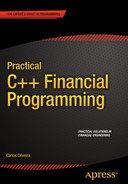
The constraints are related to the amount of money that investors want to use each year for the next five years. Since the cost of each investment is known for any of the m periods, let’s name such costs cij, for i Î {1...m} and j Î {1...n}. For each year, the investment is limited by the value Ci, the amount of capital available at time period i. Then, for each time period (where each period corresponds to one year), the constraint can be written as
Finally, we defined each variable xj as a one-or-nothing decision. That is, the variable can only assume values 1 or 0, indicating that the project will be pursued or not.
![]()
Because the problem described previously has a linear objective function and linear constraints, it is a linear optimization problem. However, the last constraint makes the problem a 0–1 integer LP problem, which can be considerably more difficult to solve than a standard LP problem.
To implement the problem described previously, I will take advantage of the MIPSolver class defined in the previous chapter. Remember that the input for any mixed integer-programming problem can be represented using a matrix of constraints, a vector or right-hand side values, and a vector of costs. Thus, we need to define these three elements when defining the desired capital allocation problem.
To give a clear demonstration of how this process works, I created a simple example that can be viewed in the member function solveProblem, which is part of the class ResourceAlloc. First, this method defines a matrix of project costs for a period of five years. We also have five projects, so this results in a square matrix—notice, however, that a square matrix is not necessary for this formulation to work.
The next few lines of the method solveProblem define the investment returns and annual budgets. An important part of this process is to use the setBinary member function, which says that each variable must have a binary value. Finally, you need to call the function solve in the MIPSolver class, which will call the Gnu Linear Programming Kit (GLPK ) solver and determine the optimum values.
The complete code for the resource allocation problem described in the previous section can be viewed in Listing 13-1. The main function at the end of the listing will instantiate the ResourceAlloc class and solve the example problem.
Listing 13-1. Cass ResourceAlloc
//
//  ResourceAlloc.h

#ifndef __FinancialSamples__ResourceAlloc__
#define __FinancialSamples__ResourceAlloc__

#include <vector>

class ResourceAlloc {
public:
    ResourceAlloc(std::vector<double> &result, double &objVal);
    ResourceAlloc(const ResourceAlloc &p);
    ~ResourceAlloc();
    ResourceAlloc &operator=(const ResourceAlloc &p);

    void solveProblem();
private:
    std::vector<double> &m_results;
    double &m_objVal;
};

#endif /* defined(__FinancialSamples__ResourceAlloc__) */

//
//  ResourceAlloc.cpp

#include "ResourceAlloc.h"

#include "LPSolver.h"
#include "Matrix.h"

#include <iostream>

using std::vector;
using std::cout;
using std::endl;

ResourceAlloc::ResourceAlloc(vector<double> &result, double &objVal)
: m_results(result),
  m_objVal(objVal)
{
}

ResourceAlloc::ResourceAlloc(const ResourceAlloc &p)
: m_results(p.m_results),
  m_objVal(p.m_objVal)
{
}

ResourceAlloc::~ResourceAlloc()
{
}

ResourceAlloc &ResourceAlloc::operator=(const ResourceAlloc &p)
{
    if (this != &p)
    {
        m_results = p.m_results;
        m_objVal = p.m_objVal;
    }
    return  *this;
}

void ResourceAlloc::solveProblem()
{
    static const double cost_array[][5] = {
        // Years:
        // 1    2   3     4    5
        {1.81, 2.4,  2.5, 0.97, 1.5},  // proj 1
        {1.29, 1.8,  2.3, 0.56, 0.5},  // proj 2
        {1.22, 1.2,  0.1, 0.48, 0 },   // proj 3
        {1.43, 1.4,  1.2, 1.2, 1.2},   // proj 4
        {1.62, 1.9,  2.5, 2.0, 1.8},   // proj 5
    };

    Matrix costs(5,5);  // cost matrix
    for (int i=0; i<5; ++i) {
        for (int j=0; j<5; ++j) {
            costs[j][i] = cost_array[i][j];
        }
    }

    vector<double> returns = {12.13, 3.95, 7.2, 4.21, 11.39};  // investment returns
    vector<double> budgets = {5.1, 6.4, 6.84, 4.5, 3.8};       // annual budgets
    MIPSolver solver(costs, budgets, returns);
    solver.setMaximization();

    for (int i=0; i<5; ++i)
    {
        solver.setColBinary(i);
    }

    // --- solve the problem
    solver.solve(m_results, m_objVal);
}

int main()
{

    vector<double> result;
    double objVal;

    ResourceAlloc ra(result, objVal);
    ra.solveProblem();
    cout << " optimum: " << objVal ;
    for (int i=0; i<result.size(); ++i)
    {
        cout << " x" << i << ": " << result[i];
    }
    cout << endl;
    return 0;
}
To run the code presented in Listing 13-1, you need to first compile it using a standards-compliant compiler such as gcc or Visual Studio. Then, you can run the resulting executable to view the results of the optimization process.
./investAllocSolver
GLPK Simplex Optimizer, v4.54
5 rows, 5 columns, 24 non-zeros
*     0: obj =   0.000000000e+00  infeas =  0.000e+00 (0)
*     5: obj =   3.209790698e+01  infeas =  0.000e+00 (0)
OPTIMAL LP SOLUTION FOUND
GLPK Integer Optimizer, v4.54
5 rows, 5 columns, 24 non-zeros
5 integer variables, all of which are binary
Integer optimization begins...
+     5: mip =     not found yet <=              +inf        (1; 0)
Solution found by heuristic: 30.72
+     6: mip =   3.072000000e+01 <=     tree is empty   0.0% (0; 1)
INTEGER OPTIMAL SOLUTION FOUND
 optimum: 30.72 x0: 1 x1: 0 x2: 1 x3: 0 x4: 1
Program ended with exit code: 0
Portfolio Optimization
Create a C++ class that can be used to define an optimal portfolio according to an LP variation of the capital asset pricing model.
Solution
One of the main uses of optimization models in finance is in the determination of investment portfolios. While there are several techniques to create balanced portfolios, the mathematical theory developed by Nobel Prize winner Harry Markowitz is the standard way to define an optimal portfolio, which is used by most financial institutions when analyzing groups of investments. In this section you will learn about the definition of portfolio optimization models using this technique of analysis, commonly referred to as modern portfolio theory.
The main goal of portfolio optimization is to create portfolios of financial assets that can provide the required investment return with a minimum of risk. For example, if the goal is to have a small return but very low risk, one can buy high-grade investments such as US treasury bills. For higher returns, one can invest in foreign or company bonds. For even higher returns, you can use stocks and exotic derivatives.
Faced with these options, and depending on an investor profile, a portfolio manager can create one or more portfolios that address the perceived client needs. For example, a more aggressive investor may request a portfolio with a larger number of high-volatility stocks, expecting therefore a higher return. Another, more conservative investor may prefer to hold bonds and stocks with lower volatility but also lower expected returns. It is also possible to combine different portfolios to achieve a mix of high and low return assets.
This type of portfolio construction strategy was studied and formalized at the end of the 1950s and became known as the capital asset pricing (CAP) model. The ideas, developed by Markowitz, used classical optimization theory to characterize the optimal solutions for such portfolio construction problems. While there is a difference between finding an optimal allocation and really achieving the desired return in the financial markets, the CAP is a very important tool for portfolio managers. It can be used, for example, to define an initial portfolio that matches a particular person’s profile, or to create financial products that target a defined long-term return (e.g., retirement portfolios for pension funds).
The mathematical formulation of the CAP can be summarized in the following way. Considering that there are n stocks and other assets in a portfolio, let xi for i Î {1..n} be the percentage of the portfolio held at investment i. Then it is clear that the sum of all such values needs to add to 1.

Also, suppose that for each investment i we have a target return ri (e.g., you can use past information as a baseline forecast). If the target return for the whole portfolio is R, then we have the following constraint:

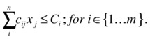
Now, in the CAP model we assume that we know the variance of each asset as well as the covariance of pairs of assets in the same portfolio. Variance is a classical measure of volatility of investments (i.e., the higher the variance, the higher the volatility). Thus, we can use the available individual volatility information to try to minimize the volatility of the whole portfolio. Since variance is a quadratic function, the objective function will also be quadratic, with individual terms depending the individual variance of individual stocks (cii) and on the covariance of pairs of stocks (cij). The resulting problem can be described as follows:


![]()
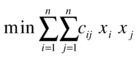
During the last few decades, many people have studied this optimization problem and its variations. The formulation employs an objective function that is quadratic (nonlinear)—that is, there are terms in the objective function that involve a multiplication of two variables. The general solution of this problem, considering this nonlinear structure, forms what is called an efficient frontier: a set of results for different combinations of portfolios, where the volatility of the target portfolio is minimized. You can see an example of efficient frontier in Figure 13-1, which shows a plot of volatility against target return. The plot is created by, at each time, fixing a desired return and then using the quadratic optimization model to find the minimum associated volatility. As you see in Figure 13-1, the plot shows that the relationship assumes the shape of a parabolic curve.
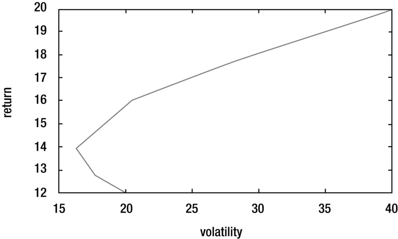
Figure 13-1. A small portion of the efficient frontier for a portfolio optimization problem
Although the quadratic model for CAP is widely used, a difficulty with it is the fact that you need a quadratic optimization solver to get results for a particular portfolio. Although several packages provide direct solutions to quadratic problems (using, for example, an interior point algorithm), GLPK is not able to solve quadratic optimization models directly. Therefore, in this section you will deal with a linearization of the original problem, which can be readily calculated using LP solvers.
This linearization was proposed in Konno and Yamazaki’s article titled “Mean-Absolute Deviation Portfolio Optimization Model and Its Applications to Tokyo Stock Market” (Management Science, vol. 37, pp. 519–529, 1991). The linearization is a modified form of the original problem that contains only linear terms in the objective function. While this is just an approximation of the original problem, in many cases it can work well enough. More important, a linearized version of the problem may be solved more quickly than the quadratic version, which may be an important consideration in some cases.
Consider the additional variables yi Î {1...T}, where T is the number of periods for the proposed investment. Then, a linear model can be described as the following:

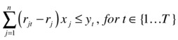
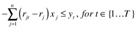


![]()
In these equations, you don’t need directly the covariance cij; instead you use the expected returns rit or investment i for period t. In other words, the idea of the model is to divide the total periods into small segments and linearize the model during that small period, taking the minimum over the complete time horizon.
With the model, which is linear, you can now create code in C++ using the LPSolver class described in the previous chapter. The new class is called ModifiedCAP and is displayed in the next section, “The Code.” The main difficulty in creating the model is defining the required input data for LPSolver, in the form of matrix A and vectors b and c. You can see how this is done in the code for member function solveModel.
The first part of the algorithm consists of setting up the required data. The vector c that defines the objective function can be easily created, since all coefficients are equal to 1.
// objective function
for (int i=m_N; i<m_N+m_T; ++i)
{
    c[i] = 1;
}
Next, the right-hand side coefficients are also simple to set up. This is true because you can move all variables yt to the left side of the inequality. Thus, most of the coefficients are zero, except for the last three.
// right-hand side vector
vector<double> b(2*m_T + 2 + 1, 0);
b[2*m_T]   =  1;
b[2*m_T+1] = -1;
b[2*m_T+2] = -m_R;
Matrix A is a little more involved but is not difficult to set up either. The main transformation you need to make is in the equality constraints. Since the problems that LPSolver considers have inequalities only, the equality is handled by converting it into two inequalities.
This makes it possible to continue to use the same simple input form used by the LPSolver (GLPK can also handle equalities directly, and you could modify the LPSolver class to do this automatically). Therefore, the following code can be used to define the input matrix A:
// matrix A
Matrix A(2*m_T + 2 + 1, m_T + m_N);
for (int i=0; i<m_T; ++i)
{
    for (int j=0; j<m_N; ++j)
    {
        A[i][j] = m_retMatrix[j][i] - m_assetRet[j];
    }
    A[i][m_N+i] = -1;
}

for (int i=m_T; i<2*m_T; ++i)
{
    for (int j=m_N; j<2*m_N; ++j)
    {
        A[i][j] = - m_retMatrix[j-m_N][i-m_T] + m_assetRet[j-m_N];
    }
    A[i][m_N+i-m_T] = -1;
}

for (int j=0; j<m_N; ++j)
{
    A[2*m_T][j]   = 1;
    A[2*m_T+1][j] = -1;
    A[2*m_T+2][j] = - m_assetRet[j];
}
The remainder of the code is just to handle constructing the LPSolver class and calling the required member functions to solve the model.
Finally, I provide a simple example of how this class could be called in practice. The sample data has four assets and five time periods. The associated expected returns are given by following matrix, which you will find in the test main function:
// sample problem: 4 assets and 5 periods

// build the expected return matrix
double val[][5] = {
    {0.051, 0.050, 0.049, 0.051, 0.05},
    {0.10, 0.099, 0.102, 0.100, 0.101},
    {0.073, 0.077, 0.076, 0.075, 0.076},
    {0.061, 0.06, 0.059, 0.061, 0.062},
};
You can view the complete code for the modified CAP in Listing 13-2. The listing contains a header and an implementation file.
Listing 13-2. Modified CAP Implementation
//
//  ModifiedCAP.h

#ifndef __FinancialSamples__ModifiedCAP__
#define __FinancialSamples__ModifiedCAP__

#include "Matrix.h"

// a modified (linearized) model for Capital Asset Pricing
class ModifiedCAP {
public:
    ModifiedCAP(int N, int T, double R, Matrix &retMatrix, const std::vector<double> &ret);
    ModifiedCAP(const ModifiedCAP &p);
    ~ModifiedCAP();
    ModifiedCAP &operator=(const ModifiedCAP &p);

    void solveModel(std::vector<double> &results, double &objVal);
private:
    int m_N;  // number of investment
    int m_T;  // number of periods
    double m_R;  // desired return
    Matrix m_retMatrix;
    std::vector<double> m_assetRet; // single returns
};

#endif /* defined(__FinancialSamples__ModifiedCAP__) */

//
//  ModifiedCAP.cpp

#include "ModifiedCAP.h"

#include "LPSolver.h"

#include <iostream>
#include <vector>

using std::vector;
using std::cout;
using std::endl;

ModifiedCAP::ModifiedCAP(int N, int T, double R, Matrix &expectedRet, const vector<double> &ret)
: m_N(N),
  m_T(T),
  m_R(R),
  m_retMatrix(expectedRet),
  m_assetRet(ret)
{
}

ModifiedCAP::ModifiedCAP(const ModifiedCAP &p)
: m_N(p.m_N),
  m_T(p.m_T),
  m_R(p.m_R),
  m_retMatrix(p.m_retMatrix),
  m_assetRet(p.m_assetRet)
{
}

ModifiedCAP::~ModifiedCAP()
{
}

ModifiedCAP &ModifiedCAP::operator=(const ModifiedCAP &p)
{
    if (this != &p)
    {
        m_N = p.m_N;
        m_T = p.m_T;
        m_R = p.m_R;
        m_retMatrix = p.m_retMatrix;
        m_assetRet = p.m_assetRet;
    }
    return *this;
}

void ModifiedCAP::solveModel(std::vector<double> &results, double &objVal)
{
    Matrix A(2*m_T + 2 + 1, m_T + m_N);
    vector<double> c(m_T + m_N, 0);

    // objective function
    for (int i=m_N; i<m_N+m_T; ++i)
    {
        c[i] = 1;
    }

    // right-hand side vector
    vector<double> b(2*m_T + 2 + 1, 0);
    b[2*m_T]   =  1;
    b[2*m_T+1] = -1;
    b[2*m_T+2] = -m_R;

    // matrix A
    for (int i=0; i<m_T; ++i)
    {
        for (int j=0; j<m_N; ++j)
        {
            A[i][j] = m_retMatrix[j][i] - m_assetRet[j];
        }
        A[i][m_N+i] = -1;
    }

    for (int i=m_T; i<2*m_T; ++i)
    {
        for (int j=m_N; j<2*m_N; ++j)
        {
            A[i][j] = - m_retMatrix[j-m_N][i-m_T] + m_assetRet[j-m_N];
        }
        A[i][m_N+i-m_T] = -1;
    }

    for (int j=0; j<m_N; ++j)
    {
        A[2*m_T][j]   = 1;
        A[2*m_T+1][j] = -1;
        A[2*m_T+2][j] = - m_assetRet[j];
    }

    LPSolver solver(A, b, c);
    solver.setMinimization();
    solver.solve(results, objVal);
}

int main()
{

    // sample problem: 4 assets and 5 periods

    // build the expected return matrix
    double val[][5] = {
        {0.051, 0.050, 0.049, 0.051, 0.05},
        {0.10, 0.099, 0.102, 0.100, 0.101},
        {0.073, 0.077, 0.076, 0.075, 0.076},
        {0.061, 0.06, 0.059, 0.061, 0.062},
    };
    Matrix retMatrix(4, 5);
    for (int i=0; i<4; ++i)
    {
        for (int j=0; j<5; ++j)
        {
            retMatrix[i][j] = val[i][j];
        }
    }

    vector<double> assetReturns = {0.05, 0.10, 0.075, 0.06};

    ModifiedCAP mc(4, 5, 0.08, retMatrix, assetReturns);

    vector<double> results;
    double objVal;
    mc.solveModel(results, objVal);

    cout << "obj value: " << objVal/5 << endl;
    for (int i=0; i<results.size(); ++i)
    {
        cout << " x" << i << ": " << results[i];
    }
    cout << endl;
}
The ModifiedCAP class presented in Listing 13-2 can be compiled using any standards-compliant C++ compiler. The main class depends on other classes presented before, such as LPSolver and Matrix. The code also depends on the GLPK library, which you can download for free as described in the previous chapter. After building this class into the executable ModifiedCap, you can run the test main function and see results similar to what is shown in the following code:
GLPK Simplex Optimizer, v4.54
13 rows, 9 columns, 46 non-zeros
      0: obj =   0.000000000e+00  infeas =  1.080e+00 (0)
*     8: obj =   3.380952381e-03  infeas =  0.000e+00 (0)
*    10: obj =   1.881151309e-03  infeas =  1.110e-16 (0)
OPTIMAL LP SOLUTION FOUND
obj value: 0.00037623
 x0: 0.320288 x1: 0.520288 x2: 0.159424 x3: 0 x4: 1.43914e-06 x5: 0 x6: 0.000879712 x7: 0.000320288 x8: 0.000679712
Program ended with exit code: 0
Looking at the output, the result shows nine LP variables. From the formulation, you will see that the first four variables correspond to the original CAP variables, while the last five are related to the time periods and therefore not used in the portfolio construction. These results tell the portfolio manager that only the first three assets should be considered in the portfolio, with percentages equal to 32%, 52%, and 15%, respectively.
To improve these results, you can modify the model accordingly to your goals. For example, you can try a different return and see how the portfolio will change based on the additional information.
Extensions to Modified CAP
Create extensions to the modified CAP model so that no asset is assigned more than 30% of the portfolio. Also, add a rule that asset classes gold and treasury bills compose at least 15% of the portfolio.
Solution
In the section “Portfolio Optimization” you saw how to create an optimization model to determine the optimal allocation of capital to a specified portfolio so that the required target return is achieved, while minimizing the volatility of the resulting portfolio. The given formulation is a modification of the original method proposed in CAP, which is a quadratic optimization model. Despite this, you can achieve quite fast results using a linear programming version of the model.
Although this model is able to cover the basis of a portfolio construction strategy, you can try other useful variations. For example, a common modification of the LP model presented previously consists of adding the minimum and maximum requirement for each asset type.
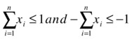
For example, suppose that you may want to increase the diversification of your portfolio by enforcing a limit on the percentage held of each asset. The main idea here is to avoid big losses that result from a portfolio concentrated in a small number of assets. Such a requirement could be easily added to the model with the following constraint:
![]()
Here, M is the desired percentage limit. When run, the LP solver will guarantee using this constraint that each percentage is not greater than the given amount M.
Similarly, you can also define a minimum amount held for each asset. In this case, it is frequently useful to have separate minimum values for each possible investment. For example, you may want to have a portfolio where treasury bills will be at least 5% at any time. If we denote the minimum required allocation by Kj, this would lead to a constraint of the type
![]()
In general, similar modifications can also be done for combinations of assets, such as treasury bills and gold. This would also work for larger groups of assets, such as adding a minimum threshold for the total number of all growth stocks in a portfolio. If you have a group of stocks L and an associated limit KL, then this general constraint can be denoted by

Finally, you can also use the idea of groups of assets to define an upper bound of the percentage held in these investments. For example, if you want to limit the percentage of a portfolio exposed to technology stocks, you can denote the group by U and the limit by KU, resulting in the following constraint:

For the benefit of simplicity, I have provided an alternative version of the ModifiedCAP class, where we have an alternative rule for diversification (at 37% level) and a minimum of 15% for the combined assets 1 and 2 (gold and treasury bills). The new code is implemented in the function solveExtendedModel, defined as
void solveExtendedModel(std::vector<double> &results, double &objVal);
The remaining parts of the class remain unchanged in this coding example.
You can find the code to solve the extended version of the CAP model in Listing 13-3. In the header file I show the complete class declaration, which is similar to the previous listing except for the added function, solveExtendedModel. The implementation file shows only the new member function, along with a test main function.
Listing 13-3. Extended Model for the CAP
//

//  ModifiedCAP.h

#ifndef __FinancialSamples__ModifiedCAP__
#define __FinancialSamples__ModifiedCAP__

#include "Matrix.h"

// a modified (linearized) model for Capital Asset Pricing
class ModifiedCAP {
public:
    ModifiedCAP(int N, int T, double R, Matrix &retMatrix, const std::vector<double> &ret);
    ModifiedCAP(const ModifiedCAP &p);
    ~ModifiedCAP();
    ModifiedCAP &operator=(const ModifiedCAP &p);

    void solveModel(std::vector<double> &results, double &objVal);
    void solveExtendedModel(std::vector<double> &results, double &objVal);
private:
    int m_N;    // number of investment
    int m_T;    // number of periods
    double m_R; // desired return
    Matrix m_retMatrix;
    std::vector<double> m_assetRet; // single returns
};

#endif /* defined(__FinancialSamples__ModifiedCAP__) */

//
//  ModifiedCAP.cpp

#include "ModifiedCAP.h"

#include "LPSolver.h"

#include <iostream>
#include <vector>

//
// ... just like code list displayed on previous section
//

void ModifiedCAP::solveExtendedModel(std::vector<double> &results, double &objVal)
{
    vector<double> c(m_T + m_N, 0);

    // objective function
    for (int i=m_N; i<m_N+m_T; ++i)
    {
        c[i] = 1;
    }

    const double M = 0.37;     // maximum of each asset
    const double K_L = 0.15;   // minimum of combined assets 1 and 2

    // right-hand side vector
    vector<double> b(2*m_T + 2 + 1 + m_N + 1 , 0);
    b[2*m_T]   =  1;
    b[2*m_T+1] = -1;
    b[2*m_T+2] = -m_R;

    for (int i=2*m_T+3; i<2*m_T + 3 + m_N; ++i)
    {
        b[i] = M;
    }
    b[2*m_T + 3 + m_N] = -K_L;

    // matrix A
    Matrix A(2*m_T + 2 + 1 + m_N + 1, m_T + m_N);
    for (int i=0; i<m_T; ++i)
    {
        for (int j=0; j<m_N; ++j)
        {
            A[i][j] = m_retMatrix[j][i] - m_assetRet[j];
        }
        A[i][m_N+i] = -1;
    }

    for (int i=m_T; i<2*m_T; ++i)
    {
        for (int j=m_N; j<2*m_N; ++j)
        {
            A[i][j] = - m_retMatrix[j-m_N][i-m_T] + m_assetRet[j-m_N];
        }
        A[i][m_N+i-m_T] = -1;
    }

    for (int j=0; j<m_N; ++j)
    {
        A[2*m_T][j]   = 1;
        A[2*m_T+1][j] = -1;
        A[2*m_T+2][j] = - m_assetRet[j];
    }

    // constraints for percentage limit
    for (int i=2*m_T+3; i<2*m_T+3+m_N; ++i)
    {
        A[i][i-(2*m_T+3)] = 1;
    }
    // constraints for assets 1 and 2
    A[2*m_T+3+m_N][0] = -1;
    A[2*m_T+3+m_N][1] = -1;

    LPSolver solver(A, b, c);
    solver.setMinimization();
    solver.solve(results, objVal);
}

int main()
{

    // sample problem: 4 assets and 5 periods

    // build the expected return matrix
    double val[][5] = {
        {0.051, 0.050, 0.049, 0.051, 0.05},
        {0.10, 0.099, 0.102, 0.100, 0.101},
        {0.073, 0.077, 0.076, 0.075, 0.076},
        {0.061, 0.06, 0.059, 0.061, 0.062},
    };
    Matrix retMatrix(4, 5);
    for (int i=0; i<4; ++i)
    {
        for (int j=0; j<5; ++j)
        {
            retMatrix[i][j] = val[i][j];
        }
    }

    vector<double> assetReturns = {0.05, 0.10, 0.075, 0.06};

    ModifiedCAP mc(4, 5, 0.08, retMatrix, assetReturns);

    vector<double> results;
    double objVal;
    mc.solveExtendedModel(results, objVal);

    cout << "obj value: " << objVal/5 << endl;
    for (int i=0; i<results.size(); ++i)
    {
        cout << " x" << i << ": " << results[i];
    }
    cout << endl;
    return 0;
}
After compiling the class described in Listing 13-3, you will be able to find the modified results of the optimized portfolio. Following is a sample output of what I achieved by adding the constraints explained previously:
./extendedModifiedCAP
GLPK Simplex Optimizer, v4.54
18 rows, 9 columns, 52 non-zeros
      0: obj = 0.000000000e+00 infeas = 1.230e+00 (0)
*    14: obj = 2.671440000e-03 infeas = 0.000e+00 (0)
OPTIMAL LP SOLUTION FOUND
obj value: 0.000534288
 x0: 0.035 x1: 0.37 x2: 0.37 x3: 0.225 x4: 1.44e-06 x5: 0.00037 x6: 0.00085 x7: 0.00026 x8: 0.00119
Program ended with exit code: 0
The solution found by the optimizer shows that the optimum allocation for the four asset classes would be 3.5%, 37%, 37%, and 22%, respectively.
Conclusion
Portfolio optimization is a tool frequently used by portfolio managers to help define a suitable capital allocation depending on the desired goals of their clients. Therefore, it is important for financial C++ programmers to be able to devise efficient solutions for such portfolio allocation problems.
In this chapter you have learned a few mathematical programming models that have been successfully used by financial institutions to create and manage portfolios as well as other financial allocation problems. In the first section you have seen how mixed-integer programming (MIP) can be used to model some financial allocation problems. You learned about some of the differences between MIP and LP models, and how they can be solved with the help of the MIPSolver class.
In the next section the focus was on the CAP model, where the main goal is to determine the percentages of each investment that need to be held in a portfolio, in order to achieve the desired outcome while at the same time minimizing the associated volatility of the investments. You have seen that although this is a quadratic programming problem, it is possible to achieve good results with a linearization of the mathematical formulation. An alternative formulation was presented and implemented in C++ using the AlternativeCAP class.
Finally, I discussed a few extensions of the basic model and how the optimization results can be understood in the context of the required portfolio. Such extensions to the basic CAP model are common, and they help in developing portfolios that are subject to real-world constraints for asset allocation.
In the next chapter, you will become acquainted with another key technique in financial engineering: Monte Carlo simulation methods. You will see a few C++ examples of how such techniques can be quickly implemented, and how the results of such methods can be interpreted.