Integrating a function is a common step in many financial algorithms. For example, some financial techniques that involve the use of differential equations depend on the evaluation of complex integrals. Such areas include derivatives pricing, insurance, and related algorithms.
However, when using these methods, you can find integrals that have no known analytical solution and need to be integrated numerically. Even if an equation can be integrated analytically, it may be more efficient to perform this task using numerical algorithms. For this purpose, this chapter explores some of the common ways of performing numerical integration. After reading this and the next chapters, you will have a better understanding of how these numerical integration algorithms work in practice and how to use them in your own projects.
Midpoint method: A simple method of integration that uses an easy-to-compute approximation based on the midpoint of each integration interval.
Trapezoid method: A more accurate method of numerical integration that employs a trapezoidal approximation to the integrated area.
Simpson’s method: A popular technique of numerical integration, Simpson’s method provides a slightly better approximation than the previous two methods.
Graphical examples of these solution methods: We present a graphical explanation of how these methods work, along with the code necessary to implement them.
The Midpoint Method
In this section, we create a C++ class to integrate functions using the midpoint method.
Solution
Integrating a function means, in a few words, finding the area of the curve formed by the function and the x-axis, when considering a single dimension. While the concept is simple, there is a large amount of literature concerning the practical importance of this problem. The most important result, also known as the fundamental theorem of calculus, is that integration is the inverse function of the derivative. In other words, applying the derivative to the integral of a function will lead to the original function. You can also integrate the derivative of a function to reach the original (up to a constant).
Finding the integral of a function by algebraic means is highly dependent on the previous definition. This means that you need to know a second function whose derivative is the function you want to integrate. In that case, the second function is the integral using the fundamental theorem of calculus. The problem is that it is not always possible to find an antiderivative using such methods. This leads to the need to determine the integral using the computational method.
There are several methods that can be used to integrate a function, but they all include the strategy of dividing the area of the desired function into many subareas and adding them all. The good thing about numerical integration is that most schemes of subdividing the area as described previously are convergent. This means that the solution for most functions can be used by any of the methods we discuss. What make these methods different is the computational effort and possibly some better convergence for a particular function or application.

Plot of function f(x)=x2+1 in the interval 1 to 5
Of course, it would be easy to solve this problem using symbolic techniques, since there is a well-known way to determine the integral of a polynomial function. However, consider how the problem could be solved using a purely computational strategy.
The goal of the algorithm is to develop an approximation so that you can determine the considered integral within a prespecified error threshold. The first step is to devise a function that could approximate the given function in the given interval. It turns out that the easiest function we can try is the constant function f(x)=c.
Suppose that we use the constant function to approximate the integral in the interval 1 to 5. We can take as the value of the constant the average value of f(x) in that interval, as determined by the extreme points.
 . Check in Figure 10-2 how this constant function
compares with the original function.
. Check in Figure 10-2 how this constant function
compares with the original function.
The original function f(x) = x2+1 compared to the constant function f(x) = c
The value of the approximation can be calculated as (5–1)10 = 40. You can compare this with the value defined by the closed calculation of the integral: the antiderivative of f(x) = x2+1 is  , and using this equation as the definite integral on the interval 1 to 5, you will find the value 45.33. From this, you see that there is a large error between the correct value and the estimation using a single midpoint calculation.
The good news is that we can improve this approximation by considering smaller intervals over the required function and adding these values together. This is the basic technique you will see in this and in the next sections. Therefore, to improve the approximation in the preceding example, we can just divide the interval 1–5 into two intervals: 1 to 3 and 3 to 5.
 for the first half of the interval and
  for the second half. This gives us an approximation of 2 × 5 + 2 × 17 = 44. Since the exact value is 45.33, you see that the approximation of 44 is much closer to the real value. You can see the new approximation in Figure 10-3.
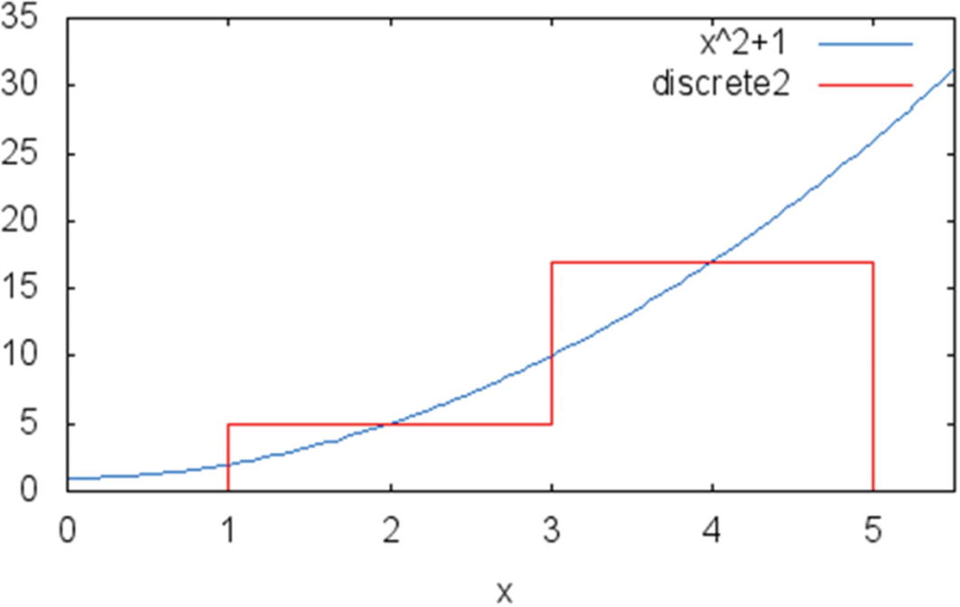
Approximating the integral of f(x) = x2+1 using two constant values
As you have seen, the secret of getting a great result from the midpoint method is subdividing the desired interval in smaller units and adding them, quite similar to the way the integral function is defined itself. While you could start with a single constant number and then divide the interval successively, it is much easier to start with a known large number of segments and expand the number of divisions if necessary. Using this strategy results in the following algorithm :
- 1.
Subdivide the initial range into N subintervals of equal sign.
- 2.
Initialize the integral value S to zero.
- 3.For each subinterval (a,b), do the following:
- a.
Take the values of a and b.
- b.
Determine the middle point value:

- c.
Add m(a,b) to the integral.
The implementation of this simple method can be found in the MidpointIntegration class .
Complete Code
Implementation for Midpoint Integration Method
Running the Code
Notice that the solution tests the approximation for two cases: when the number of intervals
is 100 (the default) and when the number of intervals is 200. Since the exact value of the function is  , this shows an improvement in the result with an error going from the third decimal place to the fourth decimal place. You can improve the approximation for different functions or required errors by increasing the number of intervals if necessary.
Trapezoid Method
In this section, we create a C++ class that implements the trapezoid method for definite integral calculation.
Solution
As you have seen in the last section, it is not difficult to come up with an approximation for the integral of a function. However, in many applications, it is useful to have a faster and more efficient way to determine the definite integral of a function. This is especially true when the function that needs to be integrated is difficult to compute in the first place. In those situations, it is better to use an approximation technique that might be able to provide more accurate solutions to the integration problem.
In this coding example, I examine an alternative way to calculate the integral of a continuous function, called the trapezoid method. As the name indicates, the trapezoid method uses a geometric, intuitive idea to render the value under the curve for a particular function, in such a way that the resulting approximation is closer to the desired value.
 to
to  . The desired integral is defined as the area under the curve. A simple approach to approximate this value is to use the area of linear function that approximates sinx between the extremes of the given interval. Using a graphical approach
, you can see the results in Figure 10-4.
. The desired integral is defined as the area under the curve. A simple approach to approximate this value is to use the area of linear function that approximates sinx between the extremes of the given interval. Using a graphical approach
, you can see the results in Figure 10-4.
Approximating the integral of f(x)=sin(x) over the interval from 1/2 to 5/2 with the help of one iteration of the trapezoid method
The trapezoid method applied to that interval gives a relatively poor approximation. The real value of the indicated integral, when computed using symbolic techniques
, is  , which is approximately 1.6787. The trapezoid method, on the other hand, yields the value
  .
.
Although this is a poor approximation, you can do better if you divide the interval of the desired function in two or more subareas. As you do this, the errors will become smaller, and the resulting value will be closer to the real value of the integral. For example, I will show how to improve the approximation of the previous function using the two subintervals from 1/2 to 3/2 and from 3/2 to 5/2.
 and
and  result in a trapezoid with an area of 0.7384. The second interval, on the other hand, has value determined by
  and
and  . The resulting trapezoid has area equal to 1.5364, which is closer to the exact value of 1.6787. You can see how this approximation works graphically in Figure 10-5.
Using the trapezoid method to approximate the area under the function f(x)=sin x, with two intervals (1/2 to 3/2 and 3/2 to 5/2)
It can be proved, as shown in the previous two examples, that as the number of subintervals is increased, the quality of the approximation gets better. As a result, you can get as close as desired from the true value of the definite integral by increasing the number of subintervals in the trapezoid method.
I present a class, called TrapezoidIntegration , which shows how to implement the trapezoid method for any function passed as an argument. The implementation is made generic with the use of the MathFunction class. Passing a new object of the desired MathFunction class , you can calculate definite integrals for different functions using the getIntegral member function.
With the TrapezoidIntegration class, you can also determine the desired number of intermediate intervals used, if you use the member function setNumIntervals . This, as a result, allows you to reduce the error in the estimates of the definite integral, if necessary. Another thing you can do using the setNumIntervals is to reduce the computational effort necessary, by reducing the number of iterations of the algorithm. In this way, you have complete control over the trade-off between degree of approximation and computational efficiency.
Complete Code
Trapezoid Integration Method
Running the Code
The program displays the value of the integral of sin(x) from 1/2 to 5/2. The approximation is given for two different settings of the number of subintervals. The first result is for 100 subintervals. The second result shows the approximation achieved when that number of subintervals is doubled.
As in the previous example, it is possible to control the quality of the approximation by increasing the number of subintervals. Also, you can reduce that number in case you prefer to get quicker results.
Using Simpson’s Method
Implement Simpson’s method for definite integral calculation.
Solution
You have seen two common ways to calculate the value of the definite integral for a given continuous function. A third method, known as Simpson’s method, is presented in this programming example. As with any technique for numeric integration, the general idea is to create a second function that approximates the desired function and apply it to several subintervals of the original domain until you get a good approximation.
Simpson’s method, unlike the previous two methods that use linear approximations to the given function, employs a second-order polynomial to achieve a better convergence. In this way, instead of relying on a linear function to achieve the desired result, the approximation proposed with Simpson’s method is better adapted to the behavior of the original curve.
The way Simpson’s method work can be easily visualized with an example. Suppose you want to integrate the function used in the previous section: f(x) = sin x. This function, being trigonometric, has no simple finite representation as a polynomial. However, it is possible to find very good approximations for a representation if you restrict the search to a small part of the function.
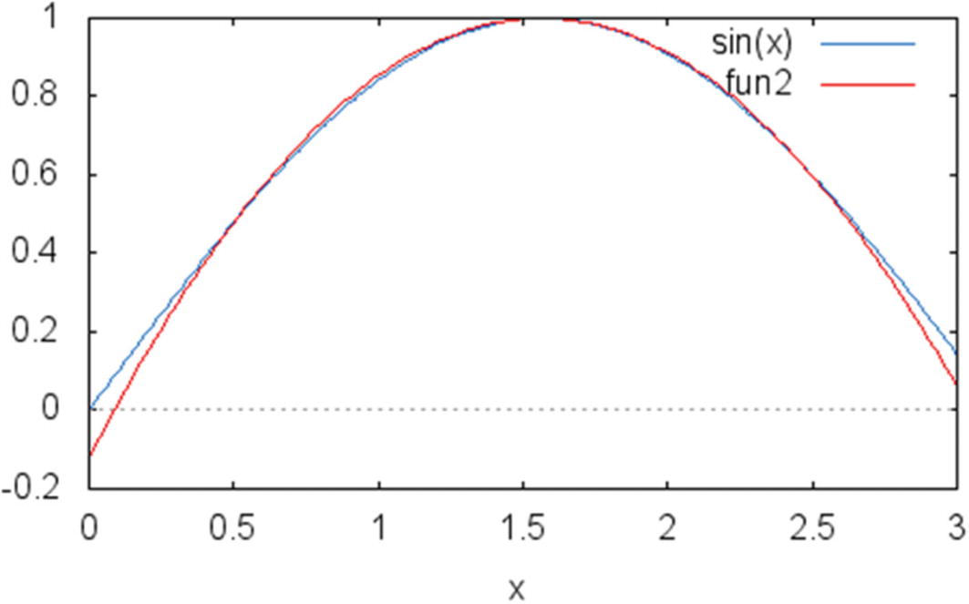
Using a second-degree polynomial to approximate the value of f(x)=sin x in the interval 1/2 to 5/2
The same idea is used in Simpson’s method. Since a quadratic approximation may be so close to the desired function, the use of quadratic functions may dramatically improve the value of the definite integral calculated in this way. In fact, experiments have shown that Simpson’s method has better accuracy than other algorithms, such as the midpoint method and the trapezoid method.
The additional accuracy of Simpson’s method can make it possible to reduce the number of subintervals necessary for the calculation of the definite integral. However, since you need to use a quadratic approximation instead of a simple linear function, the computational effort of each iteration will be higher. In the end, while Simpson’s method produces superior results for most functions, users need to be aware of a possible trade-off in terms of computational time per iteration.
![$$ frac{b-a}{6}left[f(a)+4fleft(frac{a+b}{2}
ight)+f(b)
ight] $$](https://imgdetail.ebookreading.net/202109/3/9781484268346/9781484268346__9781484268346__files__images__323908_2_En_10_Chapter__323908_2_En_10_Chapter_TeX_Equa.png)
- 1.
Define a range (A,B) where you want to calculate the integral to the equation.
- 2.
Subdivide the initial range into N subintervals of equal sign.
- 3.
Initialize the integral value S to zero.
- 4.For each subinterval (a,b), do the following:
- a.
Take the values of a and b.
- b.
Determine the approximation to the integral in the interval (a,b) given by the equation
![$$ mleft(a,b
ight)=frac{b-a}{6}left[f(a)+4fleft(frac{a+b}{2}
ight)+f(b)
ight] $$](https://imgdetail.ebookreading.net/202109/3/9781484268346/9781484268346__9781484268346__files__images__323908_2_En_10_Chapter__323908_2_En_10_Chapter_TeX_IEq15.png)
- c.
Add m(a,b) to the integral.
This algorithm has been implemented as part of SimpsonsIntegration class
Complete Code
Code for Simpson’s Integration Method
Running the Code
The code displayed in Listing 10-3 was tested using the function f(x) = sin x. The compiler used was gcc on Mac OS X and Windows. The program was tested on both platforms, generating identical results.
As you can observe from these results , the accuracy of the solution with 100 intervals is similar to the accuracy for 200 intervals. This shows that 100 subdivisions are already enough to get very good results for this technique.
Conclusion
Integrating functions is one of the basic tasks in computational mathematics, due to the great importance of integration (also known as antiderivative) as a fundamental area of calculus. In the development of financial algorithms, there are also many situations where it is necessary to find quick solutions to problems that involve the evaluation of definite integrals.
In this chapter, you have learned a few C++ programming examples that explore some of the most common techniques for numerical integration. You have seen how integration methods such as the trapezoid and Simpson’s rule can be applied to the task of finding the area under the curve for some preestablished functions.
The trapezoid method is the second important algorithm used to evaluate definite integrals. Given a general function, this method uses the function value at the extremes of the interval in order to define a trapezoid-based geometric approximation. You have seen some examples of how this strategy works, along with working code to implement the rule.
I have also discussed the well-known Simpson’s method for definite integration. Here, the approximation to the curve is performed using a quadratic equation. You saw an example of how to use polynomial equations to achieve the desired accuracy. Using Simpson’s method, you can perform integration with very good approximations, despite the fact that fewer subintervals may be necessary to read this accuracy.
Partial differential equations (PDEs) are another important mathematical tool for the financial software developer. It is important to understand how they work, as well as having tools to find solutions based on PDEs. In the next chapter, I discuss some important PDE-related techniques and their implementation in C++.