© Alejandro Serrano Mena 2019
Alejandro Serrano MenaPractical Haskellhttps://doi.org/10.1007/978-1-4842-4480-7_4

4. Using Containers and Type Classes

Alejandro Serrano Mena1 
(1)
Utrecht, The Netherlands
 

You have seen how parametric polymorphism and higher-order functions help in the process of abstraction. In this chapter, I’ll introduce a new kind of polymorphism that sits in between parametric and the absence of polymorphism: ad hoc polymorphism. Using this feature, you can express that certain types exhibit a common behavior. Incidentally, you will also learn how Haskell makes it possible to use addition, (+), on different numeric types like Integer and Float while maintaining a strong type system.

Containers will be used in the examples throughout this chapter. A container is any data structure whose purpose is to hold elements of other types in it, such as lists or trees. In addition to writing your own implementation of binary trees with a caching mechanism, you will look at implementations that are available in Hackage and Stackage , the Haskell community’s package repositories. This will lead you deeper into the features of Cabal and how you can use it to manage not only projects but also their dependencies. In addition to repositories or libraries, the Haskell community provides a lot of ways to search for code and documentation; I’ll introduce the Hoogle tool in this chapter.

While using and implementing these containers, a lot of patterns will emerge. This will be the dominant situation from now on; after looking at some useful types, you will look at their commonalities. In particular, this chapter will introduce functors, foldables, and monoids.

Using Packages

Until this point you have been using functions and data types from the base package. However, a lot of functionality is available in other packages. In this section you will first learn how to manage packages, and add them as dependencies to your projects.

A package is the distribution unit of code understood by Cabal and Stack, the tools I have already introduced for building projects. Each package is identified by a name and a version number and includes a set of modules. Optionally, the package can include some metadata such as a description or how to contact the maintainer. In fact, the projects you created previously are all packages.

You can manipulate packages by hand, but there’s an easier way to obtain and install them in your system: to make your own projects depend on them. If Cabal finds out that a package is not available in your system, it contacts the Hackage package database ( which lives at http://hackage.haskell.org ) and downloads, compiles, and installs the corresponding package. Hackage started as a mere repository for hosting packages, but now it provides some extra features such as the ability to generate documentation. Anyone with an account is allowed to upload new packages to Hackage. This ability, combined with the active Haskell community, means a wide range of libraries are available.

When your use Stack to build your projects, Hackage is not consulted by default. Instead, packages are looked for in Stackage (which lives at https://www.stackage.org ). Stackage provides snapshots of Hackage (called resolvers) in which all packages are known to work well together. This provides a huge gain for reproducibility at the expense of not always containing the bleeding-edge version of the packages.

Tip

Go to the Hackage web page and click the Packages link. Take some time to browse the different categories and the packages available in each of them. Then, find the containers package in the Data Structures category and click it. Now go the Stackage web page and click the link of the latest LTS corresponding to your version of GHC. Try to find containers in the list of packages. Compare the version of this package to the latest one available in Hackage.

In both cases, you will see the list of modules that are exported, along with its documentation. It’s important that you become comfortable with these sites because they are the main entrance to the world of Haskell libraries.

Managing Dependencies

The most common way of getting a package is not by manually downloading it but rather by adding it as a dependency of another package. You just need to add it to the property build-depends of the corresponding stanza in your .cabal file. You can add a package dependency both in the library or in executable stanzas. For example, let’s create a new project for this chapter and add the containers package as a dependency because you will use it throughout this chapter. The relevant parts of the package description file will look like this:
name:           chapter4
version:        0.1
library
  hs-source-dirs:  src
  build-depends:   base >= 4, containers
Dependencies may also specify constraints over the versions that are required. Versions are of the form a.b.c.d, with each of them being a number. The order is lexicographical; to compare two versions, the first component, a, is checked, and only if they are equal is the second is checked. If that also coincides, further components are checked in the same way. You can use any comparison operator (==, >=, >, <=, and <) and also combine them using && for conjunction and || for alternative constraints. Even though the constraint system is powerful, you should follow this rule of thumb: add a constraint requiring the minimum version where you know that your package compiles and runs (usually the version installed in your system), and another constraint to limit future versions to the next major one, that is, the next a.b in the lexicographical order. For example, at the moment of writing, the current containers version is 0.6.0.1, so the next major version would be 0.7. The suggested dependency declaration is thus as follows:
containers >= 0.6.0.1 && < 0.7

Package Versioning Policy

The meaning of the version numbers for Haskell packages has been in flux for a long time. That made it difficult to decide the range to express for a particular dependency. In Hackage, package authors are expected to adhere to the following policy:1
  • If any function, data type, type class, or instance has been changed or its type or behavior removed, the major version (i.e., the first two components) must be increased.

  • Otherwise, if only additions have been done, you can just increase the remaining components. This also holds for new modules, except in the case of a likely conflict with a module in another package.

In addition to these recommendations for package writers, the previously explained rule for specifying dependencies was introduced.

Note however that this versioning policy is a controversial issue within the Haskell community. You might find fierce arguments by defendants and opponents. But in practice, as a user of Haskell, tools work well enough even when not all packages in the repositories adhere to this practice.

As you can see, the package name and version are important parts of the project Cabal file. Furthermore, if your package is intended to be published in Hackage or publicly available in any other way, it’s important to include precise metadata. The metadata is specified by top-level properties in the package description file. The only required ones are name and version , but it’s also common to include the license, the author, the current maintainer, a small synopsis, and a larger description, the project home page, and a list of categories in which Hackage will include the package. For the chapter4 package, it might look like this:
name:           chapter4
version:        0.1
cabal-version:  >=1.2
build-type:     Simple
author:         Alejandro Serrano
synopsis:       Package for chapter 4
maintainer:     Alejandro Serrano <[email protected]>
homepage:       http://haskell.great.is

Note

You may see some extra properties, such as cabal-version and build-type. Those are meant to be used when the developer needs to tweak the building system or maintain compatibility with older versions of Cabal. My suggestion is to leave those properties as they are initially created.

Building Packages

In Chapter 2 we looked very briefly at the steps required to build a package with either of the build tools of the Haskell ecosystem, namely Cabal and Stack. In this section we look at them in more detail and describe the underlying notions in their package systems.

Building Packages with Cabal

Cabal used to be one of the very few sources of mutability in a Haskell system. All packages, including dependencies, were installed in a global location. This made the state of a Haskell installation quite brittle, especially when different packages required different versions of the same package. Fortunately, this landscape changes with the introduction of sandboxes, which isolated the dependencies of each package being developed. For a long time, sandboxes have been opt-in, and global installation remained the default method. Not any more: if you use the Cabal commands starting with new-, you use an enhanced form of sandboxes. This is now the recommended way of dealing with Haskell packaging, and it’s the one we shall describe in this section.

Since the new- commands try to isolate the package being developed from the rest of the system state, they must be run in a folder in which a .cabal file exists. This is in contrast to the previous mode of operation, in which commands could be run anywhere since they affected the global environment.

As we have discussed above, Cabal uses Hackage by default as source for our dependencies. However, the Hackage index is not consulted every time you build a package. Instead, your local Cabal installation maintains a list of all the available packages in the remote Hackage repository. Alas, this mirror of the package list is not updated automatically. You must explicitly ask Cabal to download the new version, something you should do from time to time. When using the command line, you do this by executing the cabal new-update command, as shown here:
$ cabal new-update
Downloading the latest package list from hackage.haskell.org
Now you are ready to build a package along with its dependencies. You do so by simply running cabal new-build,
$ cabal new-build
Build profile: -w ghc-8.4.3 -O1
In order, the following will be built (use -v for more details):
 - exceptions-0.10.0 (lib) (requires build)
 - ...
Downloading exceptions-0.10.0...
Configuring exceptions-0.10.0 (lib)...
...
Configuring library for chapter4-0.1...
Preprocessing library for chapter4-0.1..
Building library for chapter4-0.1..

If you get any error in this step, double check that the src folder exists.

In a first step, all the dependencies (in this example output, package exceptions version 0.10.0) are downloaded and built. Then, the package itself (in this case, chapter4) is configured and built. Of course, dependencies are only compiled in the first run, or whenever they change.

A very common scenario when developing Haskell projects is to have several packages you are developing together. Cabal can help you in that situation; the only requirement is to put all the packages in a common folder. Then create a cabal.project file with the following line:
packages: chapter4 wonderful

Then you can build one specific package by issuing the new-build command followed by the name of the package. The great benefit of using a cabal.project file is that if one of the packages depends on any other, Cabal knows where to find it. This solves one of the problems of the older behavior of Cabal, in which global mutation of the environment was the only way to develop several interdependent packages in parallel.

Building Packages with Stack

In my initial description of building packages with Stack, I hinted to the idea of resolvers. This is in fact a central idea for Stack: a resolver describes a set of packages with a specific version, and a specific compiler environment in which they work. In other words, a resolver is defined by giving a version of GHC and a version of all the packages belonging to that resolver. There are two types of resolvers: nightlies, which include newer versions but are less stable, and LTSs, which are guaranteed to work correctly. I recommend to always use an LTS for production environments.

In order to start using Stack with a Cabal project, you need to create a stack.yaml file. The main goal of that file is to specify which resolver to use. From that point on, Stack creates an isolated environment for your project, including a local version of GHC as specified by the resolver.

You don’t need to create that file by hand, though. By running stack init Stack infers which resolver to use from the current set of dependencies in your package. In particular, it tries to use the most recent LTS resolver in which all dependencies can be satisfied. Here’s the output for the chapter4 project; note how the lts-13.7 resolver is chosen.
$ stack init
Looking for .cabal or package.yaml files to use to init the project.
...
Selecting the best among 14 snapshots...
* Matches lts-13.7
Selected resolver: lts-13.7
Afterwards, you need to run stack setup . This downloads the corresponding version of GHC, if needed.
$ stack setup
Writing implicit global project config file to: ...stack.yaml
Note: You can change the snapshot via the resolver field there.
Using latest snapshot resolver: lts-13.7
Downloaded lts-13.7 build plan.
Preparing to install GHC to an isolated location.
This will not interfere with any system-level installation.
...  – downloads and installs compilers and utilities

What a waste of space, I hear you muttering. GHC is not light, indeed, and having one copy per project would result in thousands of duplicated files. Fortunately, Stack tries to share as many compilation artifacts as possible, so the same compiler is used for all the packages using the same major LTS version.

Building a package is quite similar to Cabal. Just run stack build. The main difference is that Stack takes care of updating the information about its repositories before downloading any dependencies. Then the packages are built, starting with the dependencies and ending with the package being developed.
$ stack build
exceptions-0.10.0: download
exceptions-0.10.0: configure
exceptions-0.10.0: build
exceptions-0.10.0: copy/register
chapter4-0.1.0.0: configure (lib)
Configuring chapter4-0.1.0.0...
chapter4-0.1.0.0: build (lib)
Preprocessing library for chapter4-0.1.0.0..
Building library for chapter4-0.1.0.0..
chapter4-0.1.0.0: copy/register
Installing library in <somewhere>
Registering library for chapter4-0.1.0.0..
Let’s have a look at the contents of the stack.yaml file. In your system you might find many additional comments, which are lines starting with the # symbol.
resolver: lts-13.7
packages:
- .
# extra-deps: []
The first line specifies the resolver. The packages section defines which are the folders containing the packages. By default, this section points to the folder in which the stack.yaml file resides. You can use this option to create a project with more than one package, in the same fashion as I described for Cabal. For example, you can move the file one folder up and then indicate that your folder contains both a chapter4 and a wonderful package using
packages:
- chapter4
- wonderful
The last section specifies extra dependencies, which are packages which are not available in Stackage, but are available in Hackage. Remember that Stackage provides a snapshot of Hackage, so this is a common scenario. You need to declare both the name of the package and the version. For example:
extra-deps:
- wonderful-0.2.1.0
The reason for mandating a version with every package is to keep the reproducibility guarantees of the Stack tool. Another nice ability of Stack is to point not to a package, but to a Git repository:
extra-deps:
- git: my.server/my.repo.git
  commit: a67bc8...

With all this information, you are ready to create the package for the store. Follow Exercise 4-1, and try looking carefully at all the steps needed to bring a new package to life.

Exercise 4-1: Time Machine Store Package

Create a new package that will be the origin of Time Machine Store, using either Cabal or Stack. Since it will become a web application, make it an executable. Add containers and persistent as dependencies (remember to use the version rule) and then configure and build the project. Experiment with the different metadata fields.

In addition, create both a cabal.project and a stack.yaml file. Ensure that your package builds with both tools.

Obtaining Help

I already mentioned that the Hackage and Stackage websites contains documentation about all the packages available in their databases, including module, function, type, and class descriptions. It’s a great source of information for both when you want to find information about some specific function and when you want to get a broad overview of a module. Furthermore, all the packages in the Haskell Platform come with high-quality explanations and examples.

One really cool tool that helps in daily Haskell programming is Hoogle, available at www.haskell.org/hoogle/ . The powerful Hoogle search engine allows you to search by name but also by type. Furthermore, it understands Haskell idioms. For example, if you look for a function with a specific type, it may find a more general function using a type class that the types in the signature implement, or the order of the arguments may be swapped in the found version. This tool is available also as the command-line program hoogle, which you can obtain by running cabal install hoogle in the command line. Note that this will take some time, since it needs to download and compile all dependencies in addition to the executable. Before being able to issue any query, you must run hoogle generate at the console.

Here is an example of the outcome of Hoogle for a map-like function:
$ hoogle '(a -> b) -> ([a] -> [b])'
Prelude map :: (a -> b) -> [a] -> [b]
Data.List map :: (a -> b) -> [a] -> [b]
Control.Parallel.Strategies parMap :: Strategy b -> (a -> b) -> [a] -> [b]
Control.Applicative liftA :: Applicative f => (a -> b) -> f a -> f b
Data.Traversable fmapDefault :: Traversable t => (a -> b) -> t a -> t b
Prelude fmap :: Functor f => (a -> b) -> f a -> f b
Data.Functor fmap :: Functor f => (a -> b) -> f a -> f b
# and it continues to 80 results

Containers: Maps, Sets, Trees, Graphs

In this section you will look at some container types that are common in programming. As I introduced earlier, a container is a data type whose main purpose is to hold any number of elements of a homogeneous type. In particular, you will look at maps, trees, graphs, and sets. All these structures could be implemented by using lists and tuples (e.g., you have already seen how association lists can be used to represent maps). But using specialized data types has two advantages.
  • They are much faster because they were specially developed for a particular pattern. For example, looking for the value associated to a key in a list involves searching the entire list, whereas in a map the time is almost constant.

  • Libraries implementing these structures provide functions that were created for the specific use cases of each of them. For example, you have functions for visiting nodes or getting the strongly connected components of a graph. These functions could be implemented if using lists but are not already available in the Haskell Platform.

All the containers I will talk about are provided by the containers package, so to try the examples, you need to include that package as a dependency, as in the previous section.

Maps

Let’s start with maps, which allow you to associate values with keys efficiently. No duplicate keys are allowed, so if you want to alter the value for a specific key, the new one will override the previous one. In contrast, with association lists, by implementing mappings as a list of tuples, you were responsible for maintaining such an invariant.

You’ll find the implementation of maps in the Data.Map module. However, many functions in that module collide with names from the built-in Prelude module. For that reason, you will need to qualify the module when you import it. Here you’ll qualify Data.Map by the name M, so you’ll prefix any declaration from the module with M instead of Data.Map. It’s common practice to abbreviate the qualification to a small one-letter name to write less code. In the following examples I’ll assume that the module has been imported with this line:
import qualified Data.Map as M

The type itself is Map k a. It takes as parameters the type k of the keys that will index values of type a. For example, a mapping between clients and the list of products that each client has bought will have type Map Client [Product]. In the examples you will work with simpler maps from strings to integers, which are much more concise.

In the previous chapters, I introduced the special syntax for creating lists: either using the constructor [] for an empty list or listing the elements between square brackets. Haskell has no special syntax for maps or for exporting any of its data constructors. Rather, you must create new maps either by using empty to create a map with no pairs or by using singleton, which takes a key and a value and generates a map with that single element.
*Chapter4.Containers M> M.empty
fromList []
*Chapter4.Containers M> M.singleton "hello" 3
fromList [("hello",3)]
Maps are by default shown as a list of pairs. You can convert between that style of lists and real maps by using the fromList function. If two pairs have the same key, only the last value is retained.
*Chapter4.Containers M> M.fromList [("hello",1),("bye",2),("hello",3)]
fromList [("bye",2),("hello",3)]
When inserting new values, you must remember that only one value can be associated with a specific key. This leads to two different ways in which you can proceed if a value is already associated with a key.
  • You can completely ignore that old value and just replace it with the new one. This is achieved via the insert function, which takes just the new key and value, and the map where the association must be changed, in that order.

  • You can combine the old value with the new one. To do so, use insertWith, of the following type:

    (a -> a -> a) -> k -> a -> Map k a -> Map k a

    The first parameter is the combining function that will be called with the old and new values whenever the corresponding key is already present. In some cases, you will also want to have the key as a parameter of the combining function; in that case, you should use insertWithKey, whose first parameter is of type k -> a -> a -> a. This is an instance of a common pattern in the Data.Map module; each time that a function will be called with a value of the map, there’s an alternative function ending in WithKey that also gives the key to the function.

Here’s an example of several chained insertions:
*Chapter4.Containers M> :{
*Chapter4.Containers M| let m1 = M.singleton "hello" 3
*Chapter4.Containers M|     m2 = M.insert "bye" 2 m1
*Chapter4.Containers M|     m3 = M.insert "hello" 5 m2
*Chapter4.Containers M|     m4 = M.insertWith (+) "hello" 7 m3
*Chapter4.Containers M|  in (m1,m2,m3,m4)
*Chapter4.Containers M| :}
( fromList [("hello",3)]
, fromList [("bye",2),("hello",3)]
, fromList [("bye",2),("hello",5)]
, fromList [("bye",2),("hello",12)] )

Notice how in the last step the pair ("hello",5) lived in the map and ("hello",7) was going to be inserted. You specified addition as the combinator, so you get ("hello",12) in the final map.

Note

If you come from an imperative language such as C or Java, you will be used to functions directly changing the contents of a container. By contrast, Haskell is pure, so all these functions return a new map with the corresponding change applied. However, the underlying implementation does not create a whole new copy of the data structure every time it’s changed, due to laziness (which will be explained in the next chapter). That way, performance is not compromised.

In addition to holding elements, maps are used to query by key. The null function allows you to check whether the map is empty, whereas member tells whether a specific key is available in the map. To get the associated value of a key, you can either use lookup, which returns Just value if available, or use Nothing if the key is not present. Alternatively, findWithDefault takes a value to return if the key that you query is not present. In the following interpreter session, you can see examples of what these functions do in a range of cases:
*Chapter4.Containers M> M.null M.empty
True
*Chapter4.Containers M> let m = M.fromList [("hello",3),("bye",4)]
*Chapter4.Containers M> M.null m
False
*Chapter4.Containers M> M.member "hello" m
True
*Chapter4.Containers M> M.lookup "hello" m
Just 3
*Chapter4.Containers M> M.lookup "welcome" m
Nothing
*Chapter4.Containers M> M.findWithDefault 0 "welcome" m
0
You can also delete pairs from the map, using the delete function, as shown here:
*Chapter4.Containers M> M.delete "hello" m
fromList [("bye",4)]
In addition to inserting or deleting, you can also change the value of a specific key via adjust. It takes the function that will be applied to the old value to get the new value. If the key is not present, the map is not modified.
*Chapter4.Containers M> M.adjust (+7) "hello" m
fromList [("bye",4),("hello",10)]
insert, delete, and adjust are all instances of a general function called alter that subsumes all of them. The first argument is a function of type Maybe a -> Maybe a. The input will be Nothing if the key is not already present, or it will be the previous value wrapped in a Just. What to do with that key is specified by the return value of that function. If it is Nothing, the key will be dropped, and if it is Just v, that would be the new value for the key. The following code does the same work of the previous example:
*Chapter4.Containers M> M.alter ((Just v) -> Just (v+7)) "hello" m
fromList [("bye",4),("hello",10)]

Exercise 4-2 asks you to check whether alter is a general form of the functions that were introduced earlier.

Exercise 4-2: Altering Your Maps

It’s common for Haskell libraries to contain a fully general function such as alter, which is later made more concrete in other functions. This makes it easier to work with the library. Put yourself for a moment in the place of a library designer and write the functions insert, delete, and adjust using alter.

You can also combine entire maps using union, intersection, and difference, which will produce a new map key from both maps (even if they appear in only one of them), appearing in both maps or in the first map but not the second, respectively. In the case of a key with different associated values in each map, the first map will take precedence, and its value will be used. You can have finer control by using unionWith, intersectionWith, and differenceWith, which take an extra argument that is the function that combines the elements with the same key.
*Chapter4.Containers M> :{
*Chapter4.Containers M| let m1 = M.fromList [("hello",3),("bye",4)]
*Chapter4.Containers M|     m2 = M.fromList [("hello",5),("welcome",6)]
*Chapter4.Containers M|  in (m1 `M.union` m2, M.intersectionWith (-) m1 m2)
*Chapter4.Containers M| :}
( fromList [("bye",4),("hello",3),("welcome",6)]
, fromList [("hello",-2)] )
Once you know how to operate on lists, you can usually transfer that knowledge to other data structures. In the case of maps, there are functions map, foldr, foldl, filter, and partition, among others, that have the same behavior as they have for lists but return a map. Again, for each function there’s a corresponding one suffixed by WithKey whose parameter functions also take the key that you are modifying, folding upon, or filtering. Let’s duplicate all the values in a map and then return its sum.
*Chapter4.Containers M> (M.map (*2) m, M.foldr (+) 0 m)
( fromList [("bye",8),("hello",6)], 7 )

I have already talked about converting from a list of tuples into a map using fromList. You can do the inverse transformation using assocs. You may have noticed that maps are always shown with their keys ordered. The map itself maintains that invariant, so it can easily access the maximal and minimal elements in the map. Indeed, functions such as findMin/findMax, deleteMin/deleteMax, and updateMin/updateMax take advantage of this fact and allow for fast retrieving, deleting, or updating of the values associated to those keys.

Sets

Sets are found in the Data .Set module . They behave essentially like lists but do not allow duplicates. The set of functions for this data type is virtually identical to that of maps, but only taking the value as a parameter (elements in a set don’t have a key). In the following examples, the module Data.Set will be imported qualified as S:
Prelude> import qualified Data.Set as S
You create sets with empty and singleton, much like their map counterparts. empty creates a set with no elements, and singleton creates a set with a single element. Later, you can add new elements via the insert function. The following example showcases a way to create a set with the elements "welcome" and "hello":
Prelude S> S.insert "welcome" $ S.singleton "hello"
fromList ["hello","welcome"]
Alternatively, you can create a set directly from a list of their elements using the fromList function. Duplicate elements in the list will be taken to just one, since sets can contain a sole appearance of each element.
Prelude S> S.fromList ["hello","bye","hello"]
fromList ["bye","hello"]
Similarly, there’s a toList function to convert a set to a list of its elements. The behavior of these two functions provides a way to implement the functionality of removing duplicates from a list (and also sort it in ascending order), which is actually much more performant than the nub function.
Prelude S> S.toList $ S.fromList ["duplicate","boom","duplicate"]
["boom","duplicate"]
As mentioned, the interface for Data.Set is similar to that of Data.Map. The following code shows an example of using set operations (in this case, intersection, but also union and difference are available). You can see how to check for membership with the member function. Finally, like with lists and maps, you can apply a function to each element in the set using map (but be careful because duplicate results will be compressed into just one element, and order may not be respected).
Prelude S> :{
Prelude S| let set1 = S.insert "welcome" $ S.singleton "hello"
Prelude S|     set2 = S.fromList ["hello","bye"]
Prelude S|  in ( set1 `S.intersection` set2
Prelude S|     , "welcome" `S.member` set1
Prelude S|     , S.map length set2 )
Prelude S| :}
(fromList ["hello"], True, fromList [3,5])

IntMap, IntSet, HashMap, AND HashSet

Maps can be made much more efficient if you use only integers as keys. The same happens for sets holding only integer values. For that reason, the containers library provides specific data types for that purpose, namely, IntMap and IntSet.

Alternatively, the keys on a map or the values on a set might not be integers but could be mapped almost uniquely to one integer. This mapping is called a hash of the original value. The types HashMap and HashSet in the unordered-containers package provide implementations of maps and sets whose keys and elements, respectively, can be hashed; this is much more efficient than the Map and Set types discussed in this section, if the type can to be hashed.

Like with any other value, the following containers can be nested one inside another: lists of sets, maps with string keys and values that are lists of numbers, and so on. In Exercise 4-3 you will use a map with sets as values to classify a list of clients in the store.

Exercise 4-3: Classifying Clients

For analysis purposes, it interesting to classify clients according to their type such as government organization, company, or individual. First, create a new data type to represent these kinds of clients:
data ClientKind = GovOrgKind | CompanyKind | IndividualKind
Now, create a function called classifyClients that traverses a list of clients (of type [Client Integer], with Client defined as in the previous chapter) and generates a value of type Map ClientKind (Set (Client Integer)). You should create two different implementations.
  • The first should traverse the list element by element and perform on each element the classification, decide which map item to modify, and then add itself to the set.

  • The second should first create lists corresponding to the three different kinds and at the end convert those lists to sets and generate the mentioned map from them.

You can create a large client list and run the two implementations to compare which one behaves better in speed.

Trees

Trees are composed of nodes , which hold a value and may have other trees as children. In the Data.Tree module, those children are represented as a bare list of trees, sometimes called a forest. Be aware that this representation is not specialized for any particular purpose. For some algorithms, you may want to use another kind of tree, such as AVL or red-black trees. For those cases, we have specialized packages supporting these data types, such as TreeStructures, AvlTree, and RBTree. Here’s the code defining Data.Tree.Tree:
data Tree   a = Node { rootLabel :: a, subForest :: Forest a }
type Forest a = [Tree a]
The type keyword, which I haven’t yet introduced, is used to create type synonyms, that is, to give an alternative name to a type. Usually, it’s used to call a large type by a smaller or more expressive name. For example, you can introduce the following synonym for those functions returning a Boolean value:
type Predicate a = a -> Bool

The type synonym and its expansion are interchangeable in all circumstances. That is, you can also write the type of filter as Predicate a -> [a] -> [a], and the compiler would be fine with it. In contrast, the other way to define alternative names, using newtype, doesn’t make the types equivalent. When should you use this second option will be covered later in the chapter.

As you may already know, there are several ways to visit a tree (such as traversing all of their elements), which are broadly divided in two families: depth-first traversal and breadth-first traversal. In depth-first traversal, each node of the tree recursively visits its subtrees. There’s still a choice of when to visit the value in the node itself: before any subtree (pre-order) or after all subtrees are visited (post-order). Figure 4-1 illustrates both ways of traversing a tree’s elements.
../images/316945_2_En_4_Chapter/316945_2_En_4_Fig1_HTML.jpg
Figure 4-1.

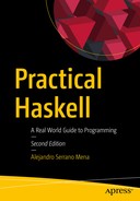
Traversing in pre-order, post-order, and breadth-first fashions

Let’s try to implement a function that traverses the tree in pre-order, applying a function to each value and returning the result in a list.
import Data.Tree
preOrder :: (a -> b) -> Tree a -> [b]
preOrder f (Node v subtrees)
  = let subtreesTraversed = concat $ map (preOrder f) subtrees
    in f v : subtreesTraversed
Notice how the code uses the map function to run the partially evaluated preOrder f on each of the subtrees. Thus, you will obtain a list of elements for each subtree, and map will return a list of lists. So, you need to flatten it to get just a single list, which is achieved using concat. Indeed, this pattern of mapping against a list and then flattening the resulting list is so common that the Prelude includes a function concatMap f, which is exactly defined as concat . map f. You can check that the function works on the tree shown in Figure 4-1.
pictureTree :: Tree Int
pictureTree = Node 1 [ Node 2 [ Node 3 []
                              , Node 4 []
                              , Node 5 [] ]
                              , Node 6 [] ]
-- In GHCi
*Chapter4.Containers> preOrder show pictureTree
["1","2","3","4","5","6"]
This pre-order traversal can be achieved using the flatten function defined in the Data.Tree module. However, it does not apply any operation of the nodes values; it just returns them as they are. The breadth-first traversal is available via the levels function, where also each level is returned as a list.
*Chapter4.Containers> flatten pictureTree
[1,2,3,4,5,6]
*Chapter4.Containers> levels pictureTree
[[1],[2,6],[3,4,5]]
Like any other container, trees in Haskell support mapping and folding over them. However, instead of functions in the same module, these operations are available through the functions fmap in Prelude and foldr in Data.Foldable. In the rest of the chapter, I will discuss why this is the case.
*Chapter4.Containers> fmap (*2) pictureTree
Node { rootLabel = 2
     , subForest = [ Node { rootLabel = 4
                          , subForest = [ Node { rootLabel = 6
                                               , subForest = [] }
                                        , Node { rootLabel = 8
                                               , subForest = [] }
                                        , Node { rootLabel = 10
                                               , subForest = [] } ] }
                   , Node { rootLabel = 12, subForest = [] } ] }
*Chapter4.Containers> Data.Foldable.foldr (+) 0 pictureTree
21

Graphs

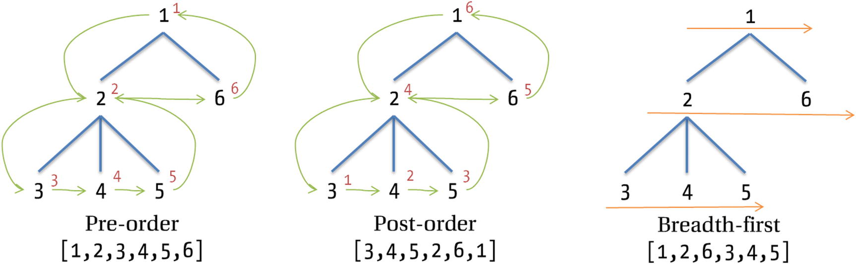
Trees are just an instance of a more general data structure called a graph. A graph is composed of a set of vertices, joined via a set of edges. In the implementation in Data.Graph, nodes are always identified by an integer, and edges are directed (an edge from a to b does not imply an edge from b to a) and without weights.

There are two ways to create a graph.
  • You use graphFromEdges when you have a list of nodes; each of them is identified by a key and holds a value, and for each node you also have its list of neighbors – that is, the list of any other nodes that receive an edge from the former. In such a case, you call graphFromEdges, which takes a list of triples, (value, key, [key]), the latest component being the aforementioned list of neighbors. In return, you get a graph but also two functions. The first one of type Vertex -> (node, key, [key]) maps a vertex identifier from the graph to the corresponding information of the node, whereas the second one, with type key -> Maybe Vertex, implements the inverse mapping: from keys to vertex identifiers.

  • If you already have your graph in a form where you have integer identifiers, you can use buildG instead. This function takes as parameters a tuple with the minimal and maximum identifiers (its bounds) and a list of tuples corresponding to each directed edge in the graph.

There is a large set of functions for inspecting the graph itself, like vertices and edges, returning the sets corresponding to their names. However, the great power of this module is the complete set of functions for walking through the elements in graphs and working with them, which are usually quite tricky to implement by hand. For example, let’s say you have a list of things to do for building a time machine. However, these tasks have some relative order. To create the door of the time machine, you first need to buy the aluminum from which it is made. This ordering can be represented using a graph, where there’s an edge from a to b if a must precede b. The following code generates the first graph in Figure 4-2:
../images/316945_2_En_4_Chapter/316945_2_En_4_Fig2_HTML.jpg
Figure 4-2.

Graphs about time machines

import Data.Graph
timeMachineGraph :: [(String, String, [String])]
timeMachineGraph =
 [("wood","wood",["walls"]), ("plastic","plastic",["walls","wheels"])
 ,("aluminum","aluminum",["wheels","door"]),("walls","walls",["done"])
 ,("wheels","wheels",["done"]),("door","door",["done"]),("done","done",[])]
timeMachinePrecedence
  :: (Graph, Vertex -> (String,String,[String]), String -> Maybe Vertex)
timeMachinePrecedence = graphFromEdges timeMachineGraph
You can build a plan for constructing the time machine by asking for a topological sort of the elements. In this sort scheme, each node n is always before any other node that receives an edge from n. Notice how in the example the mapping between vertices and keys has been used to write the results using the string representations, not the internal integer identifiers.
*Chapter4.Containers> :{
*Chapter4.Containers> let (g,v,_) = timeMachinePrecedence
*Chapter4.Containers>  in map (x -> let (k,_,_) = v x in k) $ topSort g
*Chapter4.Containers> :}
["wood","plastic","walls","aluminum","door","wheels","done"]
One detail that most of the people don’t know about time machines is that you cannot travel to any point in time with a machine. Instead, each machine has some points where you can travel, and it may be the case that you can travel to one point in only one direction. So, when performing time travel, you should be sure you are able get to the time where you want to go or that you can go back to the initial point. You can model these constraints as a graph. From each year you will have edges to each year to which you can arrive. The following code translates this idea applied to the second graph in Figure 4-2 to code:
timeMachineTravel :: Graph
timeMachineTravel = buildG (103,2013)
  [(1302,1614),(1614,1302),(1302,2013),(2013,1302),(1614,2013)
  ,(2013,1408),(1408,1993),(1408,917),(1993,917),(917,103),(103,917)]
You may ask whether you can travel from 1302 to 917; the path function will give the answer. Indeed, if you want to know every vertex that can be reached from that year, you can use reachable to find them. Let’s look at some examples starting from 1302:
*Chapter4.Containers> path timeMachineTravel 1302 917
True
*Chapter4.Containers> reachable timeMachineTravel 1302
[1302,2013,1408,917,103,1993,1614]
How can you partition the vertices such that you can always travel between all years in each set? Each component of this partition is called a strongly connected component. You can get it using scc , which will return a set of trees, each of them specifying one of those components. But if you run this function directly, you will get some enormous output. This is because when creating a graph using buildG, the library creates vertices for all identifiers in between. For that reason, you are going to filter the trees with only one node. This filtering will eliminate those vertices that were not in the initial list but also the connected components with only one element. Here’s the filtering code:
*Chapter4.Containers> filter ((Node { subForest = s }) -> s /= []) $ scc timeMachineTravel
[Node { rootLabel = 103
      , subForest = [
            Node { rootLabel = 917, subForest = []}]}
          , Node { rootLabel = 2013
                 , subForest = [
                       Node { rootLabel = 1302
                            , subForest = [
                                  Node { rootLabel = 1614
                                       , subForest = [] } ] } ] } ]
The previous output is definitely not very manageable. If instead of using buildG your graph is represented as with graphFromEdges, the output is much better. You need only to use stronglyConnComp. A special type SCC is used for representing each component. You need to run flattenSCC to obtain a printable version, as shown in the following example:
*Chapter4.Containers> map flattenSCC $ stronglyConnComp timeMachineGraph
[["done"],["door"],["walls"],["wood"],["wheels"],["plastic"],["aluminum"]]

Ad Hoc Polymorphism: Type Classes

Up to this point in the book you have seen the types of several functions in the Haskell Platform. However, if you look at some functions in the Data.Map or Data.Set module, you will find something that hasn’t yet been explained.
*Chapter4.Containers> :t M.insert
M.insert :: Ord k => k -> a -> M.Map k a -> M.Map k a

Notice how Ord k is separated from the rest of the type by => (not to be confused by the arrow -> used in the type of functions). The purpose of Ord k is to constrain the set of possible types that the k type variable can take. This is different from the parametric polymorphism of the list functions in the previous chapters. Here you ask the type to be accompanied by some functions. This kind of polymorphism is known as ad hoc polymorphism. In this case, the Ord type class is saying that the type must provide implementations of comparison operators such as < or ==. Thus, it formalizes the notion of default order that I talked about previously.

Declaring Classes and Instances

A type class (usually abbreviated as simply class) is a declaration of a set of functions along with their types, and it receives a name (in the previous case, Ord). The declaration of a type class has this syntax:
class ClassName variable where
  oneFunction   :: oneType
  ...
  otherFunction :: otherType
The variable introduced in the declaration can be used in the functions to refer to a type that supports the type class. For example, both clients and time machines have a name, so you can introduce a type class for expressing the concept “values of this type have a name” that you will call Nameable. Check how the type variable n is used in the type of the function name, as shown here:
class Nameable n where
  name :: n -> String
Now if you look at the type of name, it declares the constraint of being a Nameable.
*Chapter4.TypeClasses> :t name
name :: Nameable n => n -> String
From now on, using the name function also comes with the associated restriction, which must be specified in the corresponding type declaration . An example using Nameable could involve a function, declared outside the type class, which returns the initial of the name.
initial :: Nameable n => n -> Char
initial n = head (name n)
Of course, the main purpose of having a type class is to declare that some specific type supports the operations introduced by the class. Such a type is called an instance of a type class . The declaration of such a fact must include the implementation of the functions declared in the class.
instance ClassName Type where
  oneFunction   = ... -- implementation
  ...
  otherFunction = ... -- implementation
Following the example, the following is the instantiation of the Nameable type class by Client. Here’s a reminder of how this type looked in Chapter 3:
data Person   = Person { firstName :: String, lastName :: String }
              deriving (Show, Eq, Ord)
data Client i = GovOrg  { clientId :: i, clientName :: String }
              | Company { clientId :: i, clientName :: String
                        , person :: Person, duty :: String }
              | Individual { clientId :: i, person :: Person }
              deriving (Show, Eq, Ord)
In the instance declaration, you need to include the whole type . This means you must also write the type parameters that should be applied in the declaration (in this case, the i parameter).
instance Nameable (Client i) where
  name Individual { person = Person { firstName = f, lastName = n } }
         = f ++ " " ++ n
  name c = clientName c

Caution

Type classes in Haskell should not be confused with classes in object-oriented (OO) programming. Actually, if you had to make a connection, you can think of type classes as interfaces in those languages, but they have many more applications, such as linking together several types in a contract (e.g., specifying that an IntSet holds elements of type Int). The word instance is also used in both worlds with very different meanings. In OO languages it refers to a concrete value of a class, whereas in Haskell it refers to the implementation of a class by a type. This points to a third difference: in OO the declaration of a class includes a list of all the interfaces it implements, whereas in Haskell the declaration of a type and its implementation of a type class are separated. Indeed, in some cases they are even in different modules (these instances are referred to as orphan ones).

When you use a type that implements a class, the Haskell compiler must look for the corresponding instance declaration . It does so by looking in all the modules that are imported, independently of how they are imported. Currently, it’s not possible to prevent an instance declaration from being imported. This means that if you see some source code like the following, it may not be an error (what’s the point of having such a declaration if nothing is imported?) but rather an import of the instance declarations found in Module:
import Module ()

Exercise 4-4 shows you how to use type classes and instances. It does so in the direction of fulfilling the main target: creating a powerful time machine store.

Exercise 4-4: Prices for the Store

Besides time machines, the web store will also sell travel guides and tools for maintaining the machines. All of them have something in common: a price. Create a type class called Priceable of types supporting a price, and make those data types implement it.

The next step is creating a totalPrice function, which, given a list of things with price, computes the total amount of money to pay . The type of this function will be as follows:
totalPrice :: Priceable p => [p] -> Double

Be aware that the meaning of this signature may not match your intuition, especially if you are coming from an object-oriented programming background. When the compiler processes this code, it will look for a concrete type for the type variable p. This means it can work only with homogeneous lists. You can compute the price of a list of time machines, [TimeMachine], or a list of books, [Book]. But there’s no way to type or create a heterogeneous list containing both values of type TimeMachine and Book.

Nameable is similar to the Show type class, which provides a function called show to convert a value into a string . You have already met this type class in the definition of previous data types, but you haven’t written any instance for those data types. The reason is that Haskell can automatically write instances of a set of type classes, deriving them from the shape of the data type. This is called the deriving mechanism because the instances to generate are specified after the deriving keyword at the end of the data type definition.

Note

According to the standard, Haskell is able to derive instances for only some type classes, which are hard-coded in the compiler. However, there’s a field of functional programming, called generic programming, that provides ways to write functions that depend on the structure of data types. Chapter 14 provides an introduction to that topic.

There’s a dual class to Show , called Read , which performs the inverse function: converting a string representation into an actual value of a type, via the read function. The implementation of a Read instance is usually tricky since you must take care of spacing, proper handling of parentheses, different formats for numbers, and so forth. The good news is that Haskell also allows you to derive Read instances automatically, which are guaranteed to read back any value produced by the show function. If deriving both, you can be sure that read . show is the identity on the values of the data type; that is, the final value will be the same as the initial one.

Let’s derive Read also for the Person data type.
data Person = Person { firstName :: String, lastName  :: String }
              deriving (Show, Eq, Ord, Read)
And now let’s try to parse a string representing a person.
*Chapter4.TypeClasses> read "Person { firstName = "A", lastName = "S" }"
*** Exception: Prelude.read: no parse
The problem is that GHC has no clue about which instance of Read should be used. You haven’t specified any further operation on the result that Haskell could use to infer the final type. From the compiler point of view, the string may refer to any type. The solution is to explicitly tell what the type to be returned is. This is achieved by annotating the expression with :: followed by the type.
*Chapter4.TypeClasses> :{
*Chapter4.TypeClasses| read "Person { firstName = "A", lastName = "S" }"
*Chapter4.TypeClasses>  :: Person
*Chapter4.TypeClasses| :}
Person {firstName = "A", lastName = "S"}
Once again, you can check that Haskell infers always the most general type based on the functions used in the expressions. For example, the function read . show would work on any data type supporting both Show and Read . But in general, it also works if some data type supports Show and another one supports Read, which is more general than a single type supporting both.
*Chapter4.TypeClasses> :t read . show
read . show :: (Read c, Show a) => a -> c

Built-in Type Classes

I have spoken in the previous chapters about some list functions involving types having “default comparisons” and “default equivalences.” Now that you know about type classes, it is time to introduce the specific classes that encode those concepts, namely, Ord and Eq.

Eq is the type class declaring that a type supports checking equality (and inequality) between their values. Let’s look at its definition from the GHC source code (you can access it looking at the base package, surfing inside the Prelude module and then clicking the Source link next to the class information).
class Eq a where
    (==), (/=) :: a -> a -> Bool
    x /= y = not (x == y)
    x == y = not (x /= y)

I mentioned that type classes include only the declaration of functions to be implemented, but here you find some code implementation. The reason is that those are default definitions: code for a function that works whenever some of the rest are implemented. For example, if you implement (==), there’s a straightforward way to implement (/=), as shown earlier. When instantiating a type class, you are allowed to leave out those functions with a default implementation.

This means that when implementing Eq, you may do it without any actual implementation because all functions have default implementations. In that case, any comparison will loop forever because (/=) calls (==), which then calls (/=), and so on, indefinitely. This may lead to the program crashing out of memory or just staying unresponsive until you force its exit. For preventing such cases, type classes in Haskell usually specify a minimal complete definition; in other words, which set of functions should be implemented for the rest to work without problems? For Eq, the minimal complete definition is either (==) or (/=), so you need to implement at least one.

Caution

Knowing the minimal complete definitions for a type class is important since it’s the only way to enforce that programs behave correctly. The GHC compiler is able to check that you have defined all necessary functions from version 7.8 on. However, because this feature was not present since the beginning in the compiler, some libraries do not explicitly mention the minimal complete definition in code. Thus, you should double-check by looking at the documentation of the type class.

Given (==), you can always write (/=) as not . (==), so you may be wondering why you would include both in the type class and then have to introduce the concept of minimal complete definition? Shouldn’t (/=) be defined outside the type class? The reason for having everything in the same type class is twofold.
  • Ease of instantiation: For some types it may be more natural to write the Eq instance by defining (==), whereas in others the code for (/=) will be easier to write. Being able to do it in both ways makes it easy for consumers to instantiate the type class. This may not be so apparent for Eq, but for more complex type classes it is important.

  • Performance: Having both functions in the type classes allows you to implement the two of them if desired. This is usually done for performance reasons; maybe your type has a faster way of checking for nonequality than trying to check equality and failing.

The case of equality leads to other interesting features of Haskell’s type class system: instantiation for a type with variables and restrictions for instantiating a type class. For example, you can implement an instance of Eq for any possible list type in a generic way. You only have to check the equality element by element. However, in order to be correct, you must require the inner elements to also implement the Eq class. Let’s look at the code:
instance Eq a => Eq [a] where
  []     == []     = True
  (x:xs) == (y:ys) = x == y && xs == ys
  _      == _      = False

Let’s focus on the highlighted parts. First, there is the restriction on the elements that have been introduced using the same syntax as in functions. Then, the declaration uses a parametric [a] in the type name, with a type variable. In sum, this instance is applicable to lists of any type a that also is an Eq. The Haskell Platform already includes these declarations for many common containers, not only lists. Instances of Eq are specified for tuples, maps, sets, trees, Maybe, and so on.

As usual, the power of instantiating type classes by parametric types is not exclusive of a special set of built-in types, but it’s available for use in your own data types, as Exercise 4-5 shows.

Exercise 4-5: The Same Client

Implement Eq for the Person and Client i types introduced in the previous chapters so that it checks the equality of all the fields. Notice that for Client you may need to add some restrictions over the type of the identifiers.

The good news is that in daily work you don’t need to write those instances because Haskell can also derive Eq like it does with Show and Read .

In addition to equality, in some cases you need the notion of ordering. This is the duty of the Ord type class.
class Eq a => Ord a where
    compare              :: a -> a -> Ordering
    (<), (<=), (>), (>=) :: a -> a -> Bool
    max, min             :: a -> a -> a
    compare x y = if x == y then EQ
                  else if x <= y then LT
                  else GT
    x <  y = case compare x y of { LT -> True;  _ -> False }
    x <= y = case compare x y of { GT -> False; _ -> True }
    x >  y = case compare x y of { GT -> True;  _ -> False }
    x >= y = case compare x y of { LT -> False; _ -> True }
    max x y = if x <= y then y else x
    min x y = if x <= y then x else y

Once again, it has a lot of members, but thanks to default definitions, the minimal complete one is either implementing compare or implementing <=. However, if you look at the code in compare, you may notice that it’s using (==), which is a member of Eq. Indeed, at the beginning of the definition of Ord there’s a prerequisite for its implementation. Every type belonging to the class Ord must also belong to the class Eq. The syntax is similar again to including restrictions in functions or in instance implementations: Eq a =>.

In this case, you say that Eq is a superclass of Ord. Once again, I must warn you against any possible confusion when comparing the concept with the one in object-oriented languages. A type class does not inherit anything from its superclass but the promise that some functions will be implemented in their instances. For all the rest, they are completely different type classes. In particular, type implementations will go in separate instance declarations.

Like with Eq, Haskell provides automatic derivation of Ord instances . When doing so, it will consider that different alternatives follow the same order as in the data declaration. For example, in the declaration of clients at the beginning of the section, government organizations will always precede companies, which will always precede individuals. Then, if two values have the same constructor, Haskell will continue looking along each field in declaration order. In this case, it means that after the kind of client, the next thing to compare is its identifier. However, this may not be the best behavior, as Exercise 4-6 points out.

Exercise 4-6: Ordering Clients

The automatically derived Ord instance for Clients doesn’t make much sense. As discussed, it checks the kind of client and then its identifier. Instead of that, write a new instance with the following properties: first, the instance should compare the name of the client. Then, if they coincide, it should put individuals first and then companies and government organizations at the end. You may need to add further comparisons in the rest of the fields to make the order correct (e.g., for two companies whose responsibility fields are different, so you must decide which one to put first).

Think beforehand whether you need to include some restriction in the instance.

Other type classes you have been using are Num and its subclasses. As you may guess, Num is the class for all those types representing numbers, whether integers, rationals, or floating-point. Each subclass adds some refinement. For example, Num includes only addition, subtraction, and multiplication, but Integral adds to the mix integer division and remainders. The operations belonging to each class are summarized in Table 4-1, along with the superclass relations.
Table 4-1.

Number-Related Type Classes

Type class

Parent class

Description

Num

n/a

Basic number type. Supports addition (+), subtraction (-), multiplication (*), unary negation (negate), absolute value (abs), sign (signum), and conversion from an Integer value (fromInteger).

Real

Num

Subclass supporting conversion to Rational values (using toRational). Integer is an instance of this class because integral values can be embedded as fractions with a denominator of 1.

Integral

Real

Subclass for integer values that support integer division and integer modulus. Related functions come in triples: quot, rem, and quotRem compute the division, modulus, or both (truncating toward 0), whereas div, mod, and divMod do the truncating toward negative infinity (-∞).

Fractional

Num

Subclass for fractional values. Supports division (/), taking the reciprocal (recip) and conversion from a Rational value (fromRational).

Floating

Fractional

Subclass for floating-point values. Supports common values such as pi and e. Allows for square roots (sqrt), natural logarithms (log), exponentiation (exp for natural base and (**) for general base), and circular and hyperbolic trigonometric functions.

One of the most interesting parts in Haskell’s treatment of numbers is how it treats constants. For example, if you try to get the type of 1 in the interpreter, the result may be puzzling at first.
*Chapter4.TypeClasses> :t 1
1 :: Num a => a

As you can see, the constant itself is polymorphic. It may represent 1 in any type that instantiates Num. The reason for that is the fromInteger function, which allows you to extract a value from an integer constant.

As an example, you are going to create a data type for complex numbers and implement its Num instance.2 You may remember from your algebra class that a complex number has the form a+bi, where a is the real part and b is the imaginary part. The laws that govern their operations can be derived from the fact that i 2 =  − 1. Finally, each complex number has the concept of absolute value, |x|, and argument θx, which satisfy the condition |x|θx = x, which is exactly the one you need for abs and signum in a Num instance .
data Complex = C Double Double deriving (Show, Eq)
instance Num Complex where
  (C a1 b1) + (C a2 b2) = C (a1 + a2) (b1 + b2)
  (C a1 b1) - (C a2 b2) = C (a1 - a2) (b1 - b2)
  (C a1 b1) * (C a2 b2) = C (a1*a2-b1*b2) (a1*b2+b1*a2)
  negate (C a b)        = C (negate a) (negate b)
  fromInteger n         = C (fromInteger n) 0
  abs (C a b)           = C (sqrt $ a*a+b*b) 0
  signum c@(C a b)      = let C n _ = abs c in C (a / n) (b / n)
You have seen that type classes are a powerful tool for abstracting concepts and patterns. In the previous chapters, you looked at the default values idiom, so you may be wondering whether there’s a type class for this matter. The answer is found in the Data.Default module, in the data-default package, which provides a Default class with just one member, def, which will return the default value. If you recall the discussion in Chapter 2 about connection options, a solution using a type class would use the following, instead of connDefault:
instance Default ConnOptions where
  def = ConnOptions TCP 0 NoProxy False False NoTimeOut

Binary Trees for the Minimum Price

Until now you have saved all the information about clients in lists for this chapter. Even though you now know about where to look for already implemented types, this section is going to step back and look at the design of a custom container type that completely suits the needs of the application. In particular, the aim is to provide support for the discount module, which needs access to the cheapest elements in the container. In the process, you will see how type classes allow for a greater degree of generalization, thus increasing reusability.

In this section the container will be holding travel guides. A travel guide consists of a title, a list of authors, and a price. You can model it using a record. As you will see later, you will need some notion of less and greater than, so you need an Ord instance and with it an Eq instance.
data TravelGuide = TravelGuide { title :: String
                               , authors :: [String]
                               , price :: Double }
                 deriving (Show, Eq, Ord)

Step 1: Simple Binary Trees

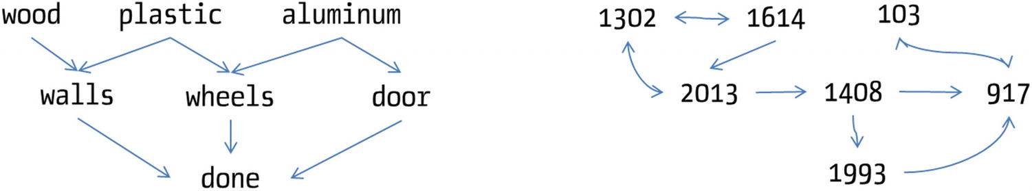
A first solution is to use bare lists. The greatest problem with them is that querying for elements in them is costly because the only option you have is to traverse the list element by element. In the worst case, you may need to traverse the entire list until you find an answer. A solution for this is to use binary trees, which have a better complexity in this task (in particular, logarithmic vs. linear).

A binary tree is a data structure made up of nodes. Each node holds a value and two references to subtrees. To indicate that a node doesn’t have some of the subtrees, you use a special leaf marker. The special property of binary trees is that any node in the left subtree will hold only those values smaller than the one in the node, whereas in the right subtree you will find values that are greater than that in the node itself. This is the reason why you need to derive Ord for the TravelGuide type. Figure 4-3 shows an example of a binary tree, with the constraints over the nodes specified in the edges.
../images/316945_2_En_4_Chapter/316945_2_En_4_Fig3_HTML.png
Figure 4-3.

Graphical example of binary tree

Now you can create the data structure of travel guide binary trees.
data BinaryTree1 = Node1 TravelGuide BinaryTree1 BinaryTree1
                 | Leaf1
                 deriving Show
As explained, searching in a binary tree is much faster because by comparing the element to look for with the node you are currently exploring, you can decide in which subtree to look, while being sure that it will never be in the other subtree.
treeFind1 :: TravelGuide -> BinaryTree1 -> Maybe TravelGuide
treeFind1 t (Node1 v l r) = case compare t v of
                              EQ -> Just v
                              LT -> treeFind1 t l
                              GT -> treeFind1 t r
treeFind1 _ Leaf1         = Nothing
You also need a way to initially create empty trees and to insert values in a tree while keeping the invariant. In the latter case, the algorithm is simple; you traverse the tree as if you were looking for the value to insert. If you reach a Leaf1, it means the value is not there and that the position for it is in the place of the leaf itself.
treeInsert1 :: TravelGuide -> BinaryTree1 -> BinaryTree1
treeInsert1 t n@(Node1 v l r) = case compare t v of
                                  EQ -> n
                                  LT -> Node1 v (treeInsert1 t l) r
                                  GT -> Node1 v l (treeInsert1 t r)
treeInsert1 t Leaf1           = Node1 t Leaf1 Leaf1

Step 2: Polymorphic Binary Trees

The basic data structure for binary trees cries out for generalization. You are not using any information inside TravelGuide for anything other than its order. This means you should work with Ord instances . The parametric version of the binary tree and its associated treeFind function now looks like this:
data BinaryTree2 a = Node2 a (BinaryTree2 a) (BinaryTree2 a)
                   | Leaf2
                   deriving Show
treeFind2 :: Ord a => a -> BinaryTree2 a -> Maybe a
treeFind2 t (Node2 v l r) = case compare t v of
                              EQ -> Just v
                              LT -> treeFind2 t l
                              GT -> treeFind2 t r
treeFind2 _ Leaf2         = Nothing

Note

You may wonder whether you can encode the restriction on the class of elements that the binary tree may hold directly in the declaration of BinaryTree2. It’s indeed possible, but it’s not recommended. The best way is to encode the restriction in each of the operations that work on that structure, as has been done in this example. Be aware that in order to impose this restriction, you must hide the Node2 and Leaf2 constructors from public consumption.

The treeFind function has been generalized, but you still need to make some changes to the treeInsert function to make it fully general. Exercise 4-7 dives into this problem.

Exercise 4-7: More Operations on Generic Trees

Make the changes needed in treeInsert to work with the new BinaryTree2.

Also, try to implement concatenation of binary trees by repeatedly inserting all the elements in one of the binary trees.

At this point, notice that the automatically derived Ord instance for TravelGuides compares first the title, then the list of authors, and finally the price. But this is not what you need; the application needs to order the travel guides by price. A first attempt would be to write a new Ord instance, like so:
instance Ord TravelGuide where
  (TravelGuide t1 a1 p1) <= (TravelGuide t2 a2 p2) =
    p1 < p2 || (p1 == p2 && (t1 < t2 || (t1 == t2 && a1 <= a2)))
Of course, you get an error about duplicate instances, as shown here:
Duplicate instance declarations:
      instance Ord TravelGuide
        -- Defined at MinimumPrice.hs:4:38
      instance Ord TravelGuide
        -- Defined at MinimumPrice.hs:6:10
A first solution is to create a one-field data type to hold travel guides by price and then create the instance for it.
data TGByPrice = TGByPrice TravelGuide
instance Ord TGByPrice where ...
The problem is that you are creating a new constructor, which at execution time must be pattern matched and unwrapped, thus taking time and hurting performance. What you need is just a way to tag values with a new type so that the compiler is able to distinguish which instance must be applied. But you want to do it without having to rewrite the initial type or having performance problems. Haskell includes a solution for this problem: a newtype declaration declares another name for an already existing type. But, in contrast to type declarations, the new name is not a synonym, but it’s viewed as a completely unrelated type. The good news is that newtype has no performance overhead because at compile time the compiler knows that values of that type will always be equal to a value of the original type, and it can delete all the constructor wrapping and pattern matching. The following code declares a newtype for TravelGuide and associates with it a new instance of the Ord type class, but now by comparing by price first:
newtype TGByPrice = TGByPrice TravelGuide deriving Eq
instance Ord TGByPrice where
  (TGByPrice (TravelGuide t1 a1 p1)) <= (TGByPrice (TravelGuide t2 a2 p2)) =
     p1 < p2 || (p1 == p2 && (t1 < t2 || (t1 == t2 && a1 <= a2)))

Let’s assume now that ordering by price is used for the rest of the examples.

Step 3: Binary Trees with Monoidal Cache

Still, finding the smallest price in the tree takes some time because you have to go into the left subtree until you reach a leaf. However, in the web page, you need to show that element often. A solution is to include a cache in every node, which stores the price of the smallest element in the tree. Let’s create a new version of binary trees, where the cache type has also been made parametric for greater generality.
data BinaryTree3 v c = Node3 v c (BinaryTree3 v c) (BinaryTree3 v c)
                     | Leaf3
                     deriving (Show, Eq, Ord)
And here’s the corresponding implementation of treeInsert, where the cache is updated at every step:
treeInsert3 :: (Ord v, Ord c)
            => v -> c -> BinaryTree3 v c -> BinaryTree3 v c
treeInsert3 v c (Node3 v2 c2 l r)
  = case compare v v2 of
      EQ -> Node3 v2 c2 l r
      LT -> Node3 v2 (min c c2) (treeInsert3 v c l) r
      GT -> Node3 v2 (min c c2) l (treeInsert3 v c r)
treeInsert3 v c Leaf3 = Node3 v c Leaf3 Leaf3

At some point you may be told that in addition to minimum prices, the marketing team wants to have information about the average price of travel guides to analyze what percentage of people are buying books under and over the average. To do this, you need to create a new insertion function, which instead of the minimum computes the sum of all the prices, so you can later divide by the total number of guides. But altogether, the structure of the function remains the same.

Let’s try to untangle the structure in both cases. What you are doing is caching some information that comes from the cached values in the subtrees and the value in the node itself. In the case of the minimal price, the operation that creates the new cached value is min, and in the case of sum, it is +. Can the exact requirements for such a function be made more precise?
  • For any two elements you need to find another one of the same type. That is, you need a function f of type c -> c -> c.

  • Also, depending on the way you have inserted elements in the tree, the structure may not be the same. But this should not matter for the final cached value. So, you need to be sure that the parentheses structure does not matter. In other words, the operation must be associative.

  • One last thing comes from the observation that when you concatenate two binary trees, you should be able to recover the new cached value for the root from the cached values from the initial roots. That means an empty tree, which contains no elements, should be assigned a value e such that f e x = f x e = x.

This structure, an associative binary operation with an element that does not affect the outcome (called a neutral element), is called a monoid and has its corresponding class in the module Data.Monoid.
class Monoid a where
  mempty  :: a            -- neutral element
  mappend :: a -> a -> a  -- associative binary operation
  mconcat :: [a] -> a
Since GHC version 8.4, Monoid is a subclass of a more general notion called Semigroup . A semigroup drops the neutral element requirement and just includes the associative binary operation.
class Semigroup a where
  (<>) :: a -> a -> a
class Semigroup a => Monoid a where ...  -- since GHC 8.4

This means that you usually won’t write mappend; rather, you can use its synonym, (<>), coming from Semigroup .

Now you can write the most general treeInsert version. Notice how in this general version you need to apply the (<>) operator both to subtrees and to the information in each node. In the version computing the minimal elements, you could take advantage from the fact that values are ordered in the tree, but in general this cannot be used.
treeInsert4 :: (Ord v, Monoid c)
            => v -> c -> BinaryTree3 v c -> BinaryTree3 v c
treeInsert4 v c (Node3 v2 c2 l r)
  = case compare v v2 of
      EQ -> Node3 v2 c2 l r
      LT -> let newLeft = treeInsert4 v c l
                newCache = c2 <> cached newLeft <> cached r
            in Node3 v2 newCache newLeft r
      GT -> let newRight = treeInsert4 v c r
                newCache = c2 <> cached l <> cached newRight
            in Node3 v2 newCache l newRight
treeInsert4 v c Leaf3 = Node3 v c Leaf3 Leaf3
cached :: Monoid c => BinaryTree3 v c -> c
cached (Node3 _ c _ _) = c
cached Leaf3           = mempty

Monoid is one of the type classes that may have multiple implementations for just one type, which has led to the creation of newtypes for some common types. Some of the most important ones are All, which implements the monoid structure of Bool under the operation (&&) with neutral element True; and All, which does the same with (||) and neutral element False. Numbers also admit two monoidal structures: Sum uses addition as an operation and 0 as a neutral element, whereas Product uses multiplication and 1.

In fact, another monoidal structure for numbers should be provided if you want to use this general cache insertion algorithm. The code needed to declare the newtype along with the new instance follows. Notice how the code uses the infinity element for floating-point, which can be obtained through 1/0.
newtype Min = Min Double deriving Show
instance Semigroup Min where
  Min x <> Min y = Min $ min x y
instance Monoid Min where
  mempty  = Min infinity where infinity = 1/0
  mappend = (<>)  -- use the definition from Semigroup

Container-Related Type Classes

In many cases while developing an application you need to change the container you are using to handle the values. So, it might be interesting to step back and think about the commonalities between them because it may be possible to abstract from them and discover some useful type class.

Functors

Let’s try to write a function applying a discount to each travel guide in a list.
modifyTravelGuidePrice
  :: Double -> [TravelGuide] -> [TravelGuide]
modifyTravelGuidePrice m  = map ( g -> tg { price = m * price tg })
And if you wanted to do it in a map or a tree, here’s how you would do that:
modifyTravelGuidePriceMap
  :: Double -> M.Map a TravelGuide -> M.Map a TravelGuide
modifyTravelGuidePriceMap m = M.map ( g -> tg { price = m * price tg })
modifyTravelGuidePriceTree
  :: Double -> T.Tree TravelGuide -> T.Tree TravelGuide
modifyTravelGuidePriceTree m = fmap ( g -> tg { price = m * price tg })
You should start seeing a pattern here; all these containers allow you to apply a function inside the data structure.
map   :: (a -> b) -> ([a]       -> [b])
M.map :: (a -> b) -> (M.Map k a -> M.Map k b)
fmap  :: (a -> b) -> (T.Tree a  -> T.Tree b)  -- version for trees
A data type supporting a function like map is called a functor. The corresponding class is defined as follows:
class Functor f where
  fmap :: (a -> b) -> f a -> f b
So, now you can write the most general function to modify the price of a travel guide.
modifyTravelGuidePrice'
  :: Functor f => Double -> f TravelGuide -> f TravelGuide
modifyTravelGuidePrice' m  = fmap ( g -> tg { price = m * price tg })

You may notice a strange fact about the Functor class; in the definition of fmap , the type variable corresponding to the instance is applied to another type variable, instead of being used raw. This means that those types that are to be functors should take one type parameter. For example, IntSet, which takes none, cannot have such an instance (even though conceptually it is a functor).

The way in which the Haskell compiler checks for the correct application of type parameters is by the kind system. Knowing it may help you make sense of some error messages. Until now, you know that values, functions, and constructors have an associated type, but types themselves are also categorized based on the level of application. To start with, all basic types such as Char or Integer have kind *. Types that need one parameter to be fully applied, such as Maybe, have kind * -> *. This syntax resembles the one used for functions on purpose. If you now have Maybe Integer, you have a type of kind * -> *, which is applied to a type of kind *. So, the final kind for Maybe Integer is indeed *.

Functor is one of the most ubiquitous type classes in Haskell. Exercise 4-8 guides you in writing the corresponding instances for one of the basic types in Haskell, Maybe, and also for the binary trees that have been introduced in the previous section.

Exercise 4-8: Functor Fun!

Write the corresponding Functor instances for both Maybe and the binary trees from the previous section. The functor instance of Maybe is quite interesting because it allows you to shorten code that just applies a function when the value is a Just (a pattern matching plus a creation of the new value is just replaced by a call to map). You will need to create a new type for Maybe values in order to make the compiler happy.

From all the binary tree types shown so far, choose BinaryTree2 as the type for instantiating Functor. In this last case, remember that you must respect the order invariant of the tree, so the best way to write the map function may involve repeatedly calling treeInsert2 on an empty tree.

Although the concept of functors came via containers, the concept is much broader. One instance of a functor that doesn’t fit that box is (->) r. The elements of this type are those functions of the form r -> a, which are functions that take as input a value of a specific type, r. Haskell syntax doesn’t help too much. In this case, just remember that a f b can also be written (f) a b if f is completely made of symbols, which is the case for ->. To begin with, let’s try to write the type for the corresponding version of fmap.
fmap :: (a -> b) -> (r -> a) -> (r -> b)
The easiest solution in this case is to apply the first function after the second to get a result of the desired type.
instance Functor ((->) r) where
  fmap f g = f . g

In this case, the concept behind the type class implementation is that of computational context. This adds to any expression an extra value of type r that can be used to control the behavior of such an expression. You will see in Chapter 6 how this mimics the existence of a constant of type r in your code.

Note

Set cannot be made an instance of Functor. The reason is that the mapping function for sets has the type Ord b => (a -> b) -> Set a -> Set b, which is not compatible with that of Functor, which doesn’t have any restriction. The Haskell language provides enough tools nowadays for creating another type class for functors that would allow Set inside it. However, this would make using the Functor type class much more complicated and would break a lot of already existing code. For that reason, the simpler version of Functor is the one included in the libraries.

Foldables

The other basic operation you can do with containers is computing some aggregate information from all the held elements, that is, a fold. This concept has its corresponding type class, called Foldable, which can be found in module Data.Foldable. To differentiate between folds and functors, you can think of folds in two different ways.
  • Like the list foldr, a fold takes an initial value and a combining function and starting with the initial value, applies the combining function to the current value and the next element in the structure.

  • You can see that a type with a binary function and some special value matches exactly the definition of a monoid. Furthermore, you have seen how combining functions in foldr should be associative, just like (<>) from Monoid is.

These two definitions allow for two different ways of instantiating the Foldable class. You need to give a definition of either foldr (the version with the combining function) or foldMap (the version with monoids).
class Foldable t where
  foldMap :: Monoid m => (a -> m) -> t a -> m
  foldr   :: (a -> b -> b) -> b -> t a -> b
  fold    :: Monoid m => t m -> m
  foldr'  :: (a -> b -> b) -> b -> t a -> b
  foldl   :: (a -> b -> a) -> a -> t b -> a
  foldl'  :: (a -> b -> a) -> a -> t b -> a
  foldr1  :: (a -> a -> a) -> t a -> a
  foldl1  :: (a -> a -> a) -> t a -> a

The rest of the operations correspond to default definitions that could be overridden for performance reasons. fold is a version of foldMap that just combines a container full of monoid values without previously applying any function. foldl corresponds to folding over the elements starting from the “other side” of the structure. You’ve already seen how the result of foldr and foldl are different if the combining function is not commutative. The versions ending with prime (') are strict versions of the functions; they will play a central role in the next chapter.

Foldables are also ubiquitous in Haskell code, like functors. Exercise 4-9 asks you to provide instances of this class for the same types you did in Exercise 4-8.

Exercise 4-9: Foldable Fun!

Maybe and binary trees can also be folded over. Write their corresponding Foldable instances. The warnings and hints from Exercise 4-8 also apply here.

As you saw in the previous chapter, a lot of different algorithms can be expressed using folds. The module Data.Foldable includes most of them, such as maximum or elem. One easy way to make your functions more general is by hiding the functions with names from the Prelude module and importing the similarly named ones using Foldable.

Note

You may wonder why Prelude includes specialized definitions for lists instead of the most general versions using Functor and Foldable. The reason is that, for a beginner, having the functions working only on [a] helps you understand the first error messages that Haskell may encounter because they don’t involve type classes. But now that you know about them, you should aim for the largest degree of abstraction that you can achieve.

In this section you wrote instances of Functor and Foldable for various data types. Because Functor and Foldable are so heavily used, the GHC developers also decided to include automatic derivation of these type classes. However, since this is not indicated in the Haskell Report, you need to enable some extensions, namely, DeriveFunctor and DeriveFoldable, for them to work. Note that if you have a type with several parameters, the one chosen for mapping or folding over is always the last one in the declaration.

Typeclassopedia

Several of the type classes discussed here, such as Monoid, Functor, and Foldable, are deeply documented in Typeclassopedia, the encyclopedia of Haskell type classes. You can find it online at wiki.haskell.org/Typeclassopedia . It’s an important source of information and examples.

Summary

In this chapter you looked at several features of the Haskell ecosystem.
  • You learned about how packages are specified as dependencies, and then used by either Cabal or Stack, allowing the reuse of many libraries already available in the repositories Hackage and Stackage.

  • Several new containers were introduced, including maps, sets, trees, and graphs. The quest for understanding their commonalities led to the discovery of the concepts of Functor and Foldable.

  • I covered the reason why (+) could work on several numeric types, namely, through ad hoc polymorphism and type classes. You learned both how to declare a new type class describing a shared concept between types and how to instantiate that class for a specific type. Furthermore, you saw how both classes and instances can depend on class constraints on other types or parameters.

  • You learned about the built-in classes Eq, describing equivalence; Ord, describing ordering; Num and its derivatives, describing numbers; and Default, describing default values for a data type.

  • I covered the design of a special binary tree with a cache, including how to incrementally improve the design of such a data type. In particular, you saw how type classes allow you to generalize the values it can take, looking specifically at the monoidal structure that is common in Haskell data types.

..................Content has been hidden....................

You can't read the all page of ebook, please click here login for view all page.
Reset
3.15.225.213