
3D Geometry
This chapter introduces the essential building blocks of 3D geometry by first extending the 2D tools from Chapters 2 and 3 to 3D. But beyond that, we will also encounter some concepts that are truly 3D, i.e., those that do not have 2D counterparts. With the geometry presented in this chapter, we will be ready to create and analyze simple 3D objects, which then could be utilized to create forms such as in Figure 8.1.
8.1 From 2D to 3D
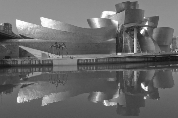
Moving from 2D to 3D geometry requires a coordinate system with one more dimension. Sketch 8.1 illustrates the [e1, e2, e3]-system that consists of the vectors
![Sketch showing the [e1, e2, e3]-axes, a point, and a vector.](http://imgdetail.ebookreading.net/math_science_engineering/24/9781466579569/9781466579569__practical-linear-algebra__9781466579569__image__158x001.png)
Thus, a vector in 3D is given as
The three components of v indicate the displacement along each axis in the [e1, e2, e3]-system. This is illustrated in Sketch 8.1. A 3D vector v is said to live in 3D space, or ℝ3, that is v ∈ ℝ3.
A point is a reference to a location. Points in 3D are given as
The coordinates indicate the point’s location in the [e1, e2, e3]-system, as illustrated in Sketch 8.1. A point p is said to live in Euclidean 3D-space, or , that is .
Let’s look briefly at some basic 3D vector properties, as we did for 2D vectors. First of all, the 3D zero vector:
Sketch 8.2 illustrates a 3D vector v along with its components. Notice the two right triangles. Applying the Pythagorean theorem twice, the length or Euclidean norm of v, denoted as ||v||, is
The length or magnitude of a 3D vector can be interpreted as distance, speed, or force.
Scaling a vector by an amount k yields ||kv|| = |k|||v||. Also, a normalized vector has unit length, ||v|| = 1.
We will get some practice working with 3D vectors. The first task is to normalize the vector
First calculate the length of v as
then the normalized vector w is
Check for yourself that ||w|| = 1.
Scale v by k = 2:
Now calculate
Thus we verified that ||2v|| = 2||v||.
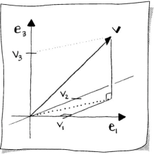
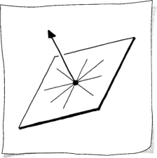
There are infinitely many 3D unit vectors. In Sketch 8.3 a few of these are drawn emanating from the origin. The sketch is a sphere of radius one.
All the rules for combining points and vectors in 2D from Section 2.2 carry over to 3D. The dot product of two 3D vectors, v and w, becomes
The cosine of the angle θ between the two vectors can be determined as
8.2 Cross Product
The dot product is a type of multiplication for two vectors that reveals geometric information, namely the angle between them. However, this does not reveal information about their orientation in relation to ℝ3. Two vectors define a plane. It would be useful to have yet another vector in order to create a 3D coordinate system that is embedded in the [e1, e2, e3]-system. This is the purpose of another form of vector multiplication called the cross product.
In other words, the cross product of v and w, written as
produces the vector u, which satisfies the following:
The vector u is perpendicular to v and w, that is
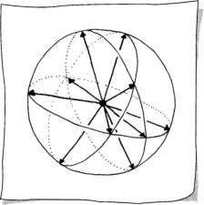
- The orientation of the vector u follows the right-hand rule. This means that if you curl the fingers of your right hand from v to w, your thumb will point in the direction of u. See Sketch 8.4.
- The magnitude of u is the area of the parallelogram defined by v and w.
Because the cross product produces a vector, it is also called a vector product.
Items 1 and 2 determine the direction of u and item 3 determines the length of u. The cross product is defined as
Item 3 ensures that the cross product of orthogonal and unit length vectors v and w results in a vector u such that u, v, w are orthonormal. In other words, u is unit length and perpendicular to v and w.
Notice that each component of (8.5) is a 2 × 2 determinant. For the ith component, omit the ith component of v and w and negate the middle determinant:
Compute the cross product of
The cross product is
Section 4.9 described why the 2 × 2 determinant, formed from two 2D vectors, is equal to the area P of the parallelogram defined by these two vectors. The analogous result for two vectors in 3D is
Recall that P is also defined by measuring a height and side length of the parallelogram, as illustrated in Sketch 8.5. The height h is
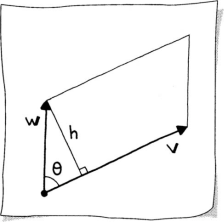
and the side length is ||v||, which makes
Equating (8.7) and (8.8) results in
Compute the area of the parallelogram formed by
Set up the cross product
Since the parallelogram is a rectangle, the area is the product of the edge lengths, so this is the correct result. Verifying (8.9),
In order to derive another useful expression in terms of the cross product, square both sides of (8.9). Thus, we have
The last line is referred to as Lagrange’s identity. We now have an expression for the area of a parallelogram in terms of a dot product.
To get a better feeling for the behavior of the cross product, let’s look at some of its properties.
- Parallel vectors result in the zero vector: v ∧ cv = 0.
- Homogeneous: cv ∧ w = c(v ∧ w).
- Antisymmetric: v ∧ w = −(w ∧ v).
- Nonassociative: u ∧ (v ∧ w) ≠ (u ∧ v) ∧ w, in general.
- Distributive: u ∧ (v + w) = u ∧ v + u ∧ w.
Right-hand rule:
Orthogonality:
Let’s test these properties of the cross product with
Make your own sketches and don’t forget the right-hand rule to guess the resulting vector direction.
Parallel vectors:
Homogeneous:
and
Antisymmetric:
Nonassociative:
which is not the same as
-
which is equal to
The cross product is an invaluable tool for engineering. One reason: it facilitates the construction of a coordinate independent frame of reference. We present two applications of this concept. In Section 8.6, outward normal vectors to a 3D triangulation, constructed using cross products, are used for rendering. In Section 20.7, a coordinate independent frame is used to move an object in space along a specified curve.
8.3 Lines
Specifying a line with 3D geometry differs a bit from 2D. In terms of points and vectors, two pieces of information define a line; however, we are restricted to specifying
- two points or
- a point and a vector parallel to the line.
The 2D geometry item (from Section 3.1), which specifies only
- a point and a vector perpendicular to the line,
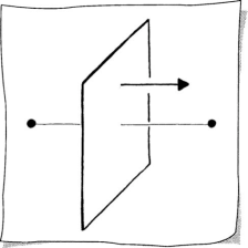
no longer works. It isn’t specific enough. (See Sketch 8.6.) In other words, an entire family of lines satisfies this specification; this family lies in a plane. (More on planes in Section 8.4.) As a consequence, the concept of a normal to a 3D line does not exist.
Let’s look at the mathematical representations of a 3D line. Clearly, from the discussion above, there cannot be an implicit form.
The parametric form of a 3D line does not differ from the 2D line except for the fact that the given information lives in 3D. A line l(t) has the form
where and . Points are generated on the line as the parameter t varies.
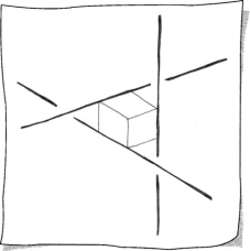
In 2D, two lines either intersect or they are parallel. In 3D this is not the case; a third possibility is that the lines are skew. Sketch 8.7 illustrates skew lines using a cube as a reference frame.
Because lines in 3D can be skew, two lines might not intersect. Revisiting the problem of the intersection of two lines given in parametric form from Section 3.8, we can see the algebraic truth in this statement. Now the two lines are
where p, and v, . To find the intersection point, we solve for t or s. Repeating (3.15), we have the linear system
However, now there are three equations and still only two unknowns. Thus, the system is overdetermined. No solution exists when the lines are skew. But we can find a best approximation, the least squares solution, and that is the topic of Section 12.7. In many applications it is important to know the closest point on a line to another line. This problem is solved in Section 11.2.
We still have the concepts of perpendicular and parallel lines in 3D.
8.4 Planes
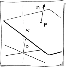
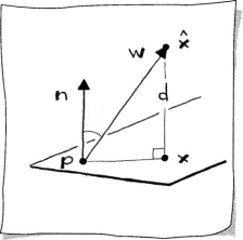
While exploring the possibility of a 3D implicit line, we encountered a plane. We’ll essentially repeat that here, however, with a little change in notation. Suppose we are given a point p and a vector n bound to p. The locus of all points x that satisfy the equation
defines the implicit form of a plane. This is illustrated in Sketch 8.8. The vector n is called the normal to the plane if ||n|| = 1. If this is the case, then (8.12) is called the point normal plane equation.
Expanding (8.12), we have
Typically, this is written as
Compute the implicit form of the plane through the point
that is perpendicular to the vector
All we need to compute is D:
Thus, the plane equation is
Similar to a 2D implicit line, if the coefficients A, B, C correspond to the normal to the plane, then |D| describes the distance of the plane to the origin. Notice in Sketch 8.8 that this is the perpendicular distance. A 2D cross section of the geometry is illustrated in Sketch 8.9. We equate two definitions of the cosine of an angle,1
and remember that the normal is unit length, to find that D = n · p.
The point normal form reflects the (perpendicular) distance of a point from a plane. This situation is illustrated in Sketch 8.10. The distance d of an arbitrary point from the point normal form of the plane is
The reason for this is precisely the same as for the implicit line in Section 3.3. See Section 11.1 for more on this topic.
Suppose we would like to find the distance of many points to a given plane. Then it is computationally more efficient to have the plane in point normal form. The new coefficients will be A′, B′, C′, D′. We normalize n in (8.12), then we may divide the implicit equation by this factor,
resulting in
Let’s continue with the plane from the previous example,
Clearly it is not in point normal form because the length of the vector
is not equal to one. In fact, .
The new coefficients of the plane equation are
resulting in the point normal plane equation,
Determine the distance d of the point
from the plane:
Notice that d > 0; this is because the point q is on the same side of the plane as the normal direction. The distance of the origin to the plane is , which is negative because it is on the opposite side of the plane to which the normal points. This is analogous to the 2D implicit line.
The implicit plane equation is wonderful for determining if a point is in a plane; however, it is not so useful for creating points in a plane. For this we have the parametric form of a plane.
The given information for defining a parametric representation of a plane usually comes in one of two ways:
- three points, or
- a point and two vectors.
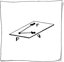
If we start with the first scenario, we choose three points p, q, r, then choose one of these points and form two vectors v and w bound to that point as shown in Sketch 8.11:
Why not just specify one point and a vector in the plane, analogous to the implicit form of a plane? Sketch 8.12 illustrates that this is not enough information to uniquely define a plane. Many planes fit that data.
Two vectors bound to a point are the data we’ll use to define a plane P in parametric form as
The two independent parameters, s and t, determine a point P(s, t) in the plane.2 Notice that (8.15) can be rewritten as
As described in Section 17.1, (1 − s − t, s, t) are the barycentric coordinates of a point P(s, t) with respect to the triangle with vertices p, q, and r, respectively.
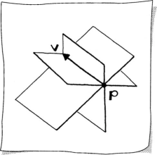
Another method for specifying a plane, as illustrated in Sketch 8.13, is as the bisector of two points. This is how a plane is defined in Euclidean geometry—the locus of points equidistant from two points. The line between two given points defines the normal to the plane, and the midpoint of this line segment defines a point in the plane. With this information it is most natural to express the plane in implicit form.
8.5 Scalar Triple Product
In Section 8.2 we encountered the area P of the parallelogram formed by vectors v and w measured as
The next natural question is how do we measure the volume of the parallelepiped, or skew box, formed by three vectors. See Sketch 8.14. The volume is a product of a face area and the corresponding height of the skew box. As illustrated in the sketch, after choosing v and w to form the face, the height is ||u|| cos θ. Thus, the volume V is
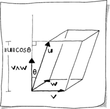
Substitute a dot product for cos θ, then
This is called the scalar triple product, and it is a number representing a signed volume.
The sign reveals something about the orientation of the three vectors. If cos θ > 0, resulting in a positive volume, then u is on the same side of the plane formed by v and w as v ∧ w. If cos θ < 0, resulting in a negative volume, then u is on the opposite side of the plane as v ∧ w. If cos θ = 0 resulting in zero volume, then u lies in this plane—the vectors are coplanar.
From the discussion above and the antisymmetry of the cross product, we see that the scalar triple product is invariant under cyclic permutations. This means that the we get the same volume for the following:
Let’s compute the volume for a parallelepiped defined by
First we compute the cross product,
then the volume V = u · y = 6. Notice that if u3 = −3, then V = −6, demonstrating that the sign of the scalar triple product reveals information about the orientation of the given vectors.
We’ll see in Section 9.5 that the parallelepiped given here is simply a rectangular box with dimensions 2 × 1 × 3 that has been sheared. Since shears preserve areas and volumes, this also confirms that the parallelepiped has volume 6.
In Section 4.9 we introduced the 2 × 2 determinant as a tool to calculate area. The scalar triple product is really just a fancy name for a 3 × 3 determinant, but we’ll get to that in Section 9.8.
8.6 Application: Lighting and Shading
Let’s look at an application of a handful of the tools that we have developed so far: lighting and shading for computer graphics. One of the most basic elements needed to calculate the lighting of a 3D object (model) is the normal, which was introduced in Section 8.4. Although a lighted model might look smooth, it is represented simply with vertices and planar facets, most often triangles. The normal of each planar facet is used in conjunction with the light source location and our eye location to calculate the lighting (color) of each vertex, and one such method is called the Phong illumination model; details of the method may be found in graphics texts such as [10, 14]. Figure 8.2 illustrates normals drawn emanating from the centroid of the facets. Determining the color of a facet is called shading. A nice example is illustrated in Figure 8.3.
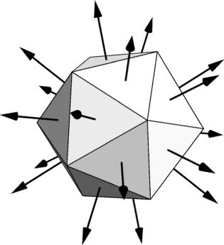
Flat shading: the normal to each planar facet is used to calculate the illumination of each facet.
We calculate the normal by using the cross product from Section 8.2. Suppose we have a triangle defined by points p, q, r. Then we form two vectors, v and w as defined in (8.14) from these points. The normal n is
The normal is by convention considered to be of unit length. Why use v ∧ w instead of w ∧ v? Triangle vertices imply an orientation. From this we follow the right-hand rule to determine the normal direction. It is important to have a rule, as just described, so the facets for a model are consistently defined. In turn, the lighting will be consistently calculated at all points on the model.
Figure 8.3 illustrates flat shading, which is the fastest and most rough-looking shading method. Each facet is given one color, so a lighting calculation is done at one point, say the centroid, based on the facet’s normal. Figure 8.4 illustrates Gouraud or smooth shading, which produces smoother-looking models but involves more calculation than flat shading. At each vertex of a triangle, the lighting is calculated. Each of these lighting vectors, ip, iq, ir, each vector indicating red, green, and blue components of light, are then interpolated across the triangle. For instance, a point x in the triangle with barycentric coordinates (u, v, w),
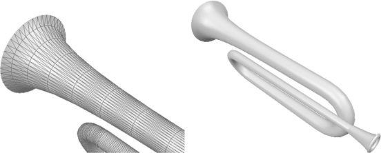
Smooth shading: a normal at each vertex is used to calculate the illumination over each facet. Left: zoomed-in and displayed with triangles. Right: the smooth shaded bugle.
will be assigned color
which is a handy application of barycentric coordinates!
Still unanswered in the smooth shading method: what normals do we assign the vertices in order to achieve a smooth shaded model? If we used the same normal at each vertex, for small enough triangles, we would wind up with (expensive) flat shading. The answer: a vertex normal is calculated as the average of the triangle normals for the triangles in the star of the vertex. (See Section 17.4 for a review of triangulations.) Better normals can be generated by weighting the contribution of each triangle normal based on the area of the triangle.
The direction of the normal n relative to our eye’s position can be used to eliminate facets from the rendering pipeline. For a closed surface, such as that in Figure 8.3, the “back-facing” facets will be obscured by the “front-facing” facets. If the centroid of a triangle is c and the eye’s position is e, then form the vector
If
then the triangle is back-facing, and we need not render it. This process is called culling. A great savings in rendering time can be achieved with culling.
Planar facet normals play an important role in computer graphics, as demonstrated in this section. For more advanced applications, consult a graphics text such as [14].

- 3D vector
- 3D point
- vector length
- unit vector
- dot product
- cross product
- right-hand rule
- orthonormal
- area
- Lagrange’s identity
- 3D line
- implicit form of a plane
- parametric form of a plane
- normal
- point normal plane equation
- point-plane distance
- plane-origin distance
- barycentric coordinates
- scalar triple product
- volume
- cyclic permutations of vectors
- triangle normal
- back-facing triangle
- lighting model
- flat and Gouraud shading
- vertex normal
- culling
8.7 Exercises
For the following exercises, use the following points and vectors:
- Normalize the vector r. What is the length of the vector 2r?
- Find the angle between the vectors v and w.
- Compute v ∧ w.
- Compute the area of the parallelogram formed by vectors v and w.
- What is the sine of the angle between v and w?
- Find three vectors so that their cross product is associative.
Are the lines
skew?
- Form the point normal plane equation for a plane through point p and with normal direction r.
- Form the point normal plane equation for the plane defined by points p, q, and r.
- Form a parametric plane equation for the plane defined by points p, q, and r.
- Form an equation of the plane that bisects the points p and q.
- Given the line l defined by point q and vector v, what is the length of the projection of vector w bound to q onto l?
- Given the line l defined by point q and vector v, what is the (perpendicular) distance of the point q + w (where w is a vector) to the line l?
- What is w ∧ 6w?
- For the plane in Exercise 8, what is the distance of this plane to the origin?
- For the plane in Exercise 8, what is the distance of the point q to this plane?
- Find the volume of the parallelepiped defined by vectors v, w, and u.
Decompose w into
where u1 and u2 are perpendicular. Additionally, find u3 to complete an orthogonal frame. Hint: Orthogonal projections are the topic of Section 2.8.
Given the triangle formed by points p, q, r, and colors
what color ic would be assigned to the centroid of this triangle using Gouraud shading? Note: the color vectors are scaled between [0, 1]. The colors black, white, red, green, blue are represented by
respectively.
1 The equations that follow should refer to p − 0 rather than simply p, but we omit the origin for simplicity.
2 This is a slight deviation in notation: an uppercase boldface letter rather than a lowercase one denoting a point.