
Eigen Things Revisited
Chapter 7 “Eigen Things” introduced the basics of eigenvalues and eigenvectors in terms of 2 × 2 matrices. But also for any n × n matrix A, we may ask if it has fixed directions and what are the corresponding eigenvalues.
In this chapter we go a little further and examine the power method for finding the eigenvector that corresponds to the dominant eigenvalue. This method is paired with an application section describing how a search engine might rank webpages based on this special eigenvector, given a fun, slang name—the Google eigenvector.
We explore “Eigen Things” of function spaces that are even more general than those in the gallery in Section 14.5.
“Eigen Things” characterize a map by revealing its action and geometry. This is key to understanding the behavior of any system. A great example of this interplay is provided by the collapse of the Tacoma Narrows Bridge in Figures 7.1 and 7.2. But “Eigen Things” are important in many other areas: characterizing harmonics of musical instruments, moderating movement of fuel in a ship, and analysis of large data sets, such as the Google matrix in Figure 15.1.
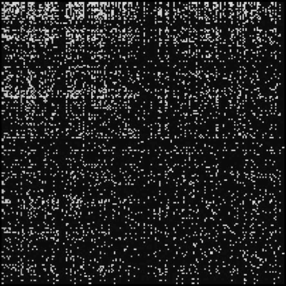
Google matrix: part of the connectivity matrix for Wikipedia pages in 2009, which is used to find the webpage ranking. (Source: Wikipedia, Google matrix.)
15.1 The Basics Revisited
If an n × n matrix A has fixed directions, then there are vectors r that are mapped to multiples λ of themselves by A. Such vectors are characterized by
or
Since r = 0 trivially satisfies this equation, we will not consider it from now on. In (15.1), we see that the matrix [A − λI] maps a nonzero vector r to the zero vector. Thus, its determinant must vanish (see Section 4.9):
The term det[A − λI] is called the characteristic polynomial of A. It is a polynomial of degree n in λ, and its zeroes are A’s eigenvalues.
Let
We find the degree four characteristic polynomial p(λ):
resulting in
The zeroes of this polynomial are found by solving p(λ) = 0. In our slightly contrived example, we find λ1 = 4, λ2 = 3, λ3 = 2, λ4 = 1. Convention orders the eigenvalues in decreasing order. Recall that the largest eigenvalue in absolute value is called the dominant eigenvalue.
Observe that this matrix is upper triangular. Forming p(λ) with expansion by minors (see Section 9.8), it is clear that the eigenvalues for this type of matrix are on the main diagonal.
We learned that Gauss elimination or LU decomposition allows us to transform a matrix into upper triangular form. However, elementary row operations change the eigenvalues, so this is not a means for finding eigenvalues. Instead, diagonalization is used when possible, and this is the topic of Chapter 16.
Here is a simple example showing that elementary row operations change the eigenvalues. Start with the matrix
that has det A = 2 and eigenvalues and . After one step of forward elimination, we have an upper triangular matrix
The determinant is invariant under forward elimination, det A′ = 2; however, the eigenvalues are not: A′ has eigenvalues λ1 = 2 and λ2 = 1.
The bad news is that one is not always dealing with upper triangular matrices like the one in Example 15.1. A general n × n matrix has a degree n characteristic polynomial
and the eigenvalues are the zeroes of this polynomial. Finding the zeroes of an nth degree polynomial is a nontrivial numerical task. In fact, for n ≥ 5, it is not certain that we can algebraically find the factorization in (15.3) because there is no general formula like we have for n = 2, the quadratic equation. An iterative method for finding the dominant eigenvalue is described in Section 15.2.
For 2 × 2 matrices, in (7.3) and (7.4), we observed that the characteristic polynomial easily reveals that the determinant is the product of the eigenvalues. For n × n matrices, we have the same situation. Consider λ = 0 in (15.3), then .
Needless to say, not all eigenvalues of a matrix are real in general. But the important class of symmetric matrices always does have real eigenvalues.
Two more properties of eigenvalues:
- The matrices A and AT have the same eigenvalues.
- Suppose A is invertible and has eigenvalues λi, then A−1 has eigenvalues 1/λi.
Having found the λi, we can now solve homogeneous linear systems
in order to find the eigenvectors ri for i = 1, n. The ri are in the null space of [A − λiI]. These are homogeneous systems, and thus have no unique solution. Oftentimes, one will normalize all eigenvectors in order to eliminate this ambiguity.
Now we find the eigenvectors for the matrix in Example 15.1. Starting with λ1 = 4, the corresponding homogeneous linear system is
and we solve it using the homogeneous linear system techniques from Section 12.3. Repeating for all eigenvalues, we find eigenvectors
For practice working with homogenous systems, work out the details. Check that each eigenvector satisfies Ari = λiri.
If some of the eigenvalues are multiple zeroes of the characteristic polynomial, for example, λ1 = λ2 = λ, then we have two identical homogeneous systems [A − λI]r = 0. Each has the same solution vector r (instead of distinct solution vectors r1, r2 for distinct eigenvalues). We thus see that repeated eigenvalues reduce the number of eigenvectors.
Let
This matrix has eigenvalues λi = 2, 2, 1. Finding the eigenvector corresponding to λ1 = λ2 = 2, we get two identical homogeneous systems
We set r3,1 = r2,1 = 1, and back substitution gives r1,1 = 5. The homogeneous system corresponding to λ3 = 1 is
Thus the two fixed directions for A are
Check that each eigenvector satisfies Ari = λiri.
Let a rotation matrix be given by
with c = cos α and s = sin α. It rotates around the e3-axis by α degrees. We should thus expect that e3 is an eigenvector—and indeed, one easily verifies that Ae3 = e3. Thus, the eigenvalue corresponding to e3 is 1.
Symmetric matrices are special again. Not only do they have real eigenvalues, but their eigenvectors are orthogonal. This can be shown in exactly the same way as we did for the 2D case in Section 7.5. Recall that in this case, A is dsaid to be diagonalizable because it is possible to transform A to the diagonal matrix Λ = R−1AR, where the columns of R are A’s eigenvectors and Λ is a diagonal matrix of A’s eigenvalues.
The symmetric matrix
has eigenvalues λ1 = 4, λ2 = 3, λ3 = 2 and corresponding eigenvectors
The eigenvalues are the diagonal elements of
and the ri are normalized for the columns of
then A is said to be diagonizable since A = RΛRT. This is the eigendecomposition of A.
Projection matrices have eigenvalues that are one or zero. A zero eigenvalue indicates that the determinant of the matrix is zero, thus a projection matrix is singular. When the eigenvalue is one, the eigenvector is projected to itself, and when the eigenvalue is zero, the eigenvector is projected to the zero vector. If λ1 = ... =λk = 1, then the column space is made up of the eigenvectors and its dimension is k, and the null space of the matrix is dimension n − k.
Define a 3 × 3 projection matrix P = uuT, where
By design, we know that this matrix is rank one and singular. The characteristic polynomial is p(λ) = λ2(1 − λ) from which we conclude that λ1 = 1 and λ2 = λ3 = 0. The eigenvector corresponding to λ1 is
and it spans the column space of P. The zero eigenvalue leads to the system
To find one eigenvector associated with this eigenvalue, we can simply assign r3 = r2 = 1, and back substitution results in r1 = −1. Alternatively, we can find two vectors that span the two dimensional null space of P,
They are orthogonal to r1. All linear combinations of elements of the null space are also in the null space, and thus r = 1r1 + 1r2. (Normally, the eigenvectors are normalized, but for simplicity they are not here.)
The trace of A is defined as
Immediately it is evident that the trace is a quick and easy way to learn a bit about the eigenvalues without computing them directly. For example, if we have a real symmetric matrix, thus real, positive eigenvalues, and the trace is zero, then the eigenvalues must all be zero. For 2 × 2 matrices, we have
thus
Example 15.8
Let
then simply by observation, we see that λ1 = −2 and λ2 = 1. Let’s compare this to the eigenvalues from (15.4). The trace is the sum of the diagonal elements, tr(A) = −1 and det A = −2. Then
resulting in the correct eigenvalues.
In Section 7.6 we introduced 2-dimensional quadratic forms, and they were easy to visualize. This idea applies to n-dimensions as well. The vector v lives in ℝn. For an n × n symmetric, positive definite matrix C, the quadratic form (7.14) becomes
where each term is paired with diagonal element ci,i and each vivj term is paired with 2ci,j due to the symmetry in C. Just as before, all terms are quadratic. Now, the contour f (v) = 1 is an n-dimensional ellipsoid. The semi-minor axis corresponds to the dominant eigenvector r1 and its length is , and the semi-major axis corresponds to rn and its length is.
A real matrix is positive definite if
for any nonzero vector v in ℝn. This means that the quadratic form is positive everywhere except for v = 0. This is the same condition we encountered in (7.17).
15.2 The Power Method
Let A be a symmetric n × n matrix.1 Further, let the eigenvalues of A be ordered such that |λ1| ≥ |λ2| ≥ ... ≥ |λn|. Then λ1 is called the dominant eigenvalue of A. To simplify the notation to come, refer to this dominant eigenvalue as λ, and let r be its corresponding eigenvector. In Section 7.7, we considered repeated applications of a matrix; we restricted ourselves to the 2D case. We encountered an equation of the form
which clearly holds for matrices of arbitrary size. This equation may be interpreted as follows: if A has an eigenvalue λ, then Ai has an eigenvalue λi with the same corresponding eigenvector r.
This property may be used to find the dominant eigenvalue and eigenvector. Consider the vector sequence
where r(1) is an arbitrary (nonzero) vector.
After a sufficiently large i, the r(i) will begin to line up with r, as illustrated in the two leftmost examples in Figure 15.2. Here is how to utilize that fact for finding λ: for sufficiently large i, we will approximately have
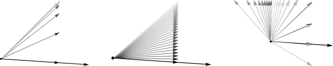
The power method: three examples whose matrices are given in Example 15.9. The longest black vector is the initial (guess) eigenvector. Successive iterations are in lighter shades of gray. Each iteration is scaled with respect to the ∞-norm.
This means that all components of r(i+1) and r(i) are (approximately) related by
In the algorithm to follow, rather than checking each ratio, we will use the ∞-norm to define λ upon each iteration.
Algorithm:
Initialization:
- Estimate dominant eigenvector r(1) ≠ 0.
- Find j where and set .
- Set λ(1) = 0.
- Set tolerance ε.
- Set maximum number of iterations m.
For k = 2, ..., m,
- y = Ar(k−1),
- λ(k) = yj.
- Find j where |yj| = ||y||∞.
- If yj = 0 then output: “eigenvalue zero; select new r(1) and restart”; exit.
- r(k) = y/yj.
- If |λ(k) − λ(k−1) | < ε then output: λ(k) and r(k); exit.
- If k = m output: “maximum iterations exceeded.”
Some remarks on using this method:
- If |λ| is either “large” or “close” to zero, the r(k) will either become unbounded or approach zero in length, respectively. This has the potential to cause numerical problems. It is prudent, therefore, to scale the r(k), so in the algorithm above, at each step, the eigenvector is scaled by its element with the largest absolute value—with respect to the ∞-norm.
- Convergence seems impossible if r(1) is perpendicular to r, the eigenvector of λ. Theoretically, no convergence will kick in, but for once numerical round-off is on our side: after a few iterations, r(k) will not be perpendicular to r and we will converge—if slowly!
- Very slow convergence will also be observed if .
- The power method as described here is limited to symmetric matrices with one dominant eigenvalue. It may be generalized to more cases, but for the purpose of this exposition, we decided to outline the principle rather than to cover all details.
Figure 15.2 illustrates three cases, A1, A2, A3, from left to right. The three matrices and their eigenvalues are as follows:
and for all of them, we used
In all three examples, the vectors r(i) were scaled relative to the ∞-norm, thus r(1) is scaled to
An ε tolerance of 5.0 × 10⁻⁴ was used for each matrix.
The first matrix, A1 is symmetric and the dominant eigenvalue is reasonably separated from λ2, hence the rapid convergence in 11 iterations. The estimate for the dominant eigenvalue: λ = 2.99998.
The second matrix, A2, is also symmetric, however λ1 is close in value to λ2, hence convergence is slower, needing 41 iterations. The estimate for the dominant eigenvalue: λ = 2.09549.
The third matrix, a rotation matrix that is not symmetric, has complex eigenvalues, hence no convergence. By following the change in gray scale, we can follow the path of the iterative eigenvector estimate. The wide variation in eigenvectors makes clear the outline of the ∞-norm. (Consult Figure 13.2 for an illustration of unit vectors with respect to the ∞-norm.)
A more realistic numerical example is presented next with the Google eigenvector.
15.3 Application: Google Eigenvector
We now study a linear algebra aspect of search engines. While many search engine techniques are highly proprietary, they all share the basic idea of ranking webpages. The concept was first introduced by S. Brin and L. Page in 1998, and forms the basis of the search engine Google. Here we will show how ranking webpages is essentially a straightforward eigenvector problem.
The web (at some frozen point in time) consists of N webpages, most of them pointing to (having links to) other webpages. A page that is pointed to very often would be considered important, whereas a page with none or only very few other pages pointing to it would be considered not important. How can we rank all webpages according to how important they are? In the sequel, we assume all webpages are ordered in some fashion (such as lexicographic) so we can assign a number, such as i, to each page.
First, two definitions: if page i points to page j, then we say this is an outlink for page i, whereas if page j points to page i, then this is an inlink for page i. A page is not supposed to link to itself. We can represent this connectivity structure of the web by an N × N adjacency matrix C: Each outlink for page i is recorded by setting Cj,i = 1. If page i does not have an outlink to page j, then cj,i = 0.
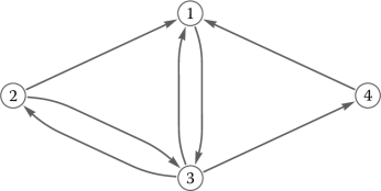
An example matrix is the following:
In this example, page 1 has one outlink since c3,1 = 1 and three inlinks since c1,2 = c1,3 = c1,4 = 1. Thus, the ith column describes the outlinks of page i and the ith row describes the inlinks of page i. This connectivity structure is illustrated by the directed graph of Figure 15.3.
The ranking ri of any page i is entirely defined by C. Here are some rules with increasing sophistication:
- The ranking ri should grow with the number of page i’s inlinks.
- The ranking ri should be weighted by the ranking of each of page i’s inlinks.
- Let page i have an inlink from page j. Then the more outlinks page j has, the less it should contribute to ri.
Let’s elaborate on these rules. Rule 1 says that a page that is pointed to very often deserves high ranking. But rule 2 says that if all those inlinks to page i prove to be low-ranked, then their sheer number is mitigated by their low rankings. Conversely, if they are mostly high-ranked, then they should boost page i’s ranking. Rule 3 implies that if page j has only one outlink and it points to page i, then page i should be “honored” for such trust from page j. Conversely, if page j points to a large number of pages, page i among them, this does not give page i much pedigree.
Although not realistic, assume for now that each page as at least one outlink and at least one inlink so that the matrix C is structured nicely. Let oi represent the total number of outlinks of page i. This is simply the sum of all elements of the ith column of C. The more outlinks page i has, the lower its contribution to page j’s ranking it will have. Thus we scale every element of column i by 1/oi. The resulting matrix D with
is called the Google matrix. Note that all columns of D have nonnegative entries and sum to one. Matrices with that property (or with respect to the rows) are called stochastic.2
In our example above, we have
We note that finding ri involves knowing the ranking of all pages, including ri. This seems like an ill-posed circular problem, but a little more analysis leads to the following matrix problem. Using the vector r = [r1, ..., rN]T, one can find
This states that we are looking for the eigenvector of D corresponding to the eigenvalue 1. But how do we know that D does indeed have an eigenvalue 1? The answer is that all stochastic matrices have that property. One can even show that 1 is D’s largest eigenvalue. This vector r is called a stationary vector.
To find r, we simply employ the power method from Section 15.2. This method needs an initial guess for r, and setting all ri = 1, which corresponds to equal ranking for all pages, is not too bad for that. As the iterations converge, the solution is found. The entries of r are real, since they correspond to a real eigenvalue.
The vector r now contains the ranking of every page, called page rank by Google. If Google retrieves a set of pages all containing a link to a term you are searching for, it presents them to you in decreasing order of the pages’ ranking.
Back to our 4 × 4 example from above: D has an eigenvalue 1 and the corresponding eigenvector
which was calculated with the power method algorithm in Section 15.2. Notice that r3 = 1 is the largest component, therefore page 3 has the highest ranking. Even though pages 1 and 3 have the same number of inlinks, the solitary outlink from page 1 to page 3 gives page 3 the edge in the ranking.
In the real world, in 2013, there were approximately 50 billion webpages. This was the world’s largest matrix to be used ever. Luckily, it contains mostly zeroes and thus is extremely sparse. Without taking advantage of that, Google (and other search engines) could not function. Figure 15.1 illustrates a portion of a Google matrix for approximately 3 million pages. We gave three simple rules for building D, but in the real world, many more rules are needed. For example, webpages with no inlinks or outlinks must be considered. We would want to modify D to ensure that the ranking r has only nonnegative components. In order for the power method to converge, other modifications of D are required as well, but that topic falls into numerical analysis.
15.4 Eigenfunctions
An eigenvalue λ of a matrix A is typically thought of as a solution of the matrix equation
In Section 14.5, we encountered more general spaces than those formed by finite-dimensional vectors: those are spaces formed by polynomials. Now, we will even go beyond that: we will explore the space of all real-valued functions. Do eigenvalues and eigenvectors have meaning there? Let’s see.
Let f be a function, meaning that y = f (x) assigns the output value y to an input value x, and we assume both x and y are real numbers. We also assume that f is smooth, or differentiable. An example might be f (x) = sin(x).
The set of all such functions f forms a linear space as observed in Section 14.5.
We can define linear maps L for elements of this function space. For example, setting L f = 2 f is such a map, albeit a bit trivial. A more interesting linear map is that of taking derivatives: D f = f′. Thus, to any function f, the map D assigns another function, namely the derivative of f. For example, let f (x) = sin(x). Then D f (x) = cos(x).
How can we marry the concept of eigenvalues and linear maps such as D? First of all, D will not have eigenvectors, since our linear space consists of functions, not vectors. So we will talk of eigenfunctions instead. A function f is an eigenfunction of D (or any other linear map) if it is mapped to a multiple of itself:
The scalar multiple λ is, as usual, referred to as an eigenvalue of f. Note that D may have many eigenfunctions, each corresponding to a different λ.
Since we know that D means taking derivatives, this becomes
Any function f satisfying (15.11) is thus an eigenfunction of the derivative map D.
Now you have to recall your calculus: the function f (x) = ex satisfies
which may be written as
Hence 1 is an eigenvalue of the derivative map D. More generally, all functions f (x) = eλx satisfy (for λ ≠ 0):
which may be written as
Hence all real numbers λ ≠ 0 are eigenvalues of D, and the corresponding eigenfunctions are eλx. We see that our map D has infinitely many eigenfunctions!
Let’s look at another example: the map is the second derivative, L f = f″. A set of eigenfunctions for this map is cos(kx) for k = 1, 2, ... since
and the eigenvalues are −k2. Can you find another set of eigenfunctions?
This may seem a bit abstract, but eigenfunctions actually have many uses, for example in differential equations and mathematical physics. In engineering mathematics, orthogonal functions are key for applications such as data fitting and vibration analysis. Some well- known sets of orthogonal functions arise as the result of the solution to a Sturm-Liouville equation such as
This is a linear second order differential equation with boundary conditions, and it defines a boundary value problem. Unknown are the functions y(x) that satisfy this equation. Solving this boundary value problem is out of the scope of this book, so we simply report that y(x) = sin(ax) for a = 1, 2, .... These are eigenfunctions of (15.13) and the corresponding eigenvalues are λ = a2.

- eigenvalue
- eigenvector
- characteristic polynomial
- eigenvalues and eigenvectors of a symmetric matrix
- dominant eigenvalue
- eigendecomposition
- trace
- quadratic form
- positive definite matrix
- power method
- max-norm
- adjacency matrix
- directed graph
- stochastic matrix
- stationary vector
- eigenfunction
15.5 Exercises
What are the eigenvalues and eigenvectors for
What are the eigenvalues and eigenvectors for
Find the eigenvalues of the matrix
If
is an eigenvector of
what is the corresponding eigenvalue?
The matrices A and AT have the same eigenvalues. Why?
If A has eigenvalues 4, 2, 0, what is the rank of A? What is the determinant?
Suppose a matrix A has a zero eigenvalue. Will forward elimination change this eigenvalue?
Let a rotation matrix be given by
which rotates around the e2-axis by −α degrees. What is one eigenvalue and eigenvector?
For the matrix
show that the determinant equals the product of the eigenvalues and the trace equals the sum of the eigenvalues.
What is the dominant eigenvalue in Exercise 9?
Compute the eigenvalues of A and A2 where
Let A be the matrix
carry out three steps of the power method with (15.7), and use r(3) and r(4) in (15.8) to estimate A’s dominant eigenvalue. If you are able to program, then try implementing the power method algorithm.
Let A be the matrix
Starting with the vector
carry out three steps of the power method with (15.7), and use r(3) and r(4) in (15.8) to estimate A’s dominant eigenvalue. If you are able to program, then try implementing the power method algorithm.
Of the following matrices, which one(s) are stochastic matrices?
The directed graph in Figure 15.4 describes inlinks and outlinks to webpages. What is the corresponding adjacency matrix C and stochastic (Google) matrix D?
For the adjacency matrix
draw the corresponding directed graph that describes these inlinks and outlinks to webpages. What is the corresponding stochastic matrix D?
The Google matrix in Exercise 16 has dominant eigenvalue 1 and corresponding eigenvector r = [1/5, 2/5, 14/15, 2/5, 1]T. Which page has the highest ranking? Based on the criteria for page ranking described in Section 15.3, explain why this is so.
Find the eigenfunctions and eigenvalues for L f (x) = xf′.
For the map L f = f″, a set of eigenfunctions is given in (15.12). Find another set of eigenfunctions.
1The method discussed in this section may be extended to nonsymmetric matrices, but since those eigenvalues may be complex, we will avoid them here.
2More precisely, matrices for which the columns sum to one are called left stochastic. If the rows sum to one, the matrix is right stochastic and if the rows and columns sum to one, the matrix is doubly stochastic.