
General Linear Spaces
In Sections 4.3 and 9.2, we had a first look at the concept of linear spaces, also called vector spaces, by examining the properties of the spaces of all 2D and 3D vectors. In this chapter, we will provide a framework for linear spaces that are not only of dimension two or three, but of possibly much higher dimension. These spaces tend to be somewhat abstract, but they are a powerful concept in dealing with many real-life problems, such as car crash simulations, weather forecasts, or computer games. The linear space of cubic polynomials over [0, 1] is important for many applications. Figure 14.1 provides an artistic illustration of some of the elements of this linear space. Hence the term “general” in the chapter title refers to the dimension and abstraction that we will study.
![Figure showing general linear spaces: all cubic polynomials over the interval [0, 1] form a linear space. Some elements of this space are shown.](http://imgdetail.ebookreading.net/math_science_engineering/24/9781466579569/9781466579569__practical-linear-algebra__9781466579569__image__303x001.png)
General linear spaces: all cubic polynomials over the interval [0, 1] form a linear space. Some elements of this space are shown.
14.1 Basic Properties of Linear Spaces
We denote a linear space of dimension n by . The elements of are vectors, denoted (as before) by boldface letters such as u or v. We need two operations to be defined on the elements of : addition and multiplication by a scalar such as s or t. With these operations in place, the defining property for a linear space is that any linear combination of vectors,
results in a vector in the same space. This is called the linearity property. Note that both s and t may be zero, asserting that every linear space has a zero vector in it. This equation is familiar to us by now, as we first encountered it in Section 2.6, and linear combinations have been central to working in the linear spaces of ℝ2 and ℝ3.1
But in this chapter, we want to generalize linear spaces; we want to include new kinds of vectors. For example, our linear space could be the quadratic polynomials or all 3 × 3matrices. Because the objects in the linear space are not always in the format of what we traditionally call a vector, we choose to call these linear spaces, which focuses on the linearity property rather than vector spaces. Both terms are accepted. Thus, we will expand our notation for objects of a linear space—we will not always use boldface vector notation. In this section, we will look at just a few examples of linear spaces, more examples of linear spaces will appear in Section 14.5.
Let’s start with a very familiar example of a linear space: ℝ2. Suppose
are elements of this space; we know that
is also in ℝ2.
Let the linear space be the set of all 2 × 2 matrices. We know that the linearity property (14.1) holds because of the rules of matrix arithmetic from Section 4.12.
Let’s define to be all vectors w in ℝ2 that satisfy w2 ≥ 0. For example, e1 and e2 live in . Is this a linear space?
It is not: we can form a linear combination as in (14.1) and produce
which is not in .
In a linear space let’s look at a set of r vectors, where 1 ≤ r ≤ n. A set of vectors v1,...,vr is called linearly independent if it is impossible to express one of them as a linear combination of the others. For example, the equation
will not have a solution set s2,..., sr in case the vectors v1,...,vr are linearly independent. As a simple consequence, the zero vector can be expressed only in a trivial manner in terms of linearly independent vectors, namely if
then s1 = ... = sr = 0. If the zero vector can be expressed as a nontrivial combination of r vectors, then we say these vectors are linearly dependent.
If the vectors v1,...,vr are linearly independent, then the set of all vectors that may be expressed as a linear combination of them forms a subspace of , of dimension r. We also say this subspace is spanned by v1, ..., vr. If this subspace equals the whole space , then we call v1, ..., vn a basis for , If is a linear space of dimension n, then any n +1 vectors in it are linearly dependent.
Let’s consider one very familiar linear space: ℝ3. A commonly used basis forℝ3 are the linearly independent vectors e1, e2, e3. A linear combination of these basis vectors, for example,
is also in ℝ3. Then the four vectors v e1, e2, e3 are linearly dependent.
Any one of the four vectors forms a one-dimensional subspace of ℝ3. Since v and each of the ei are linearly independent, any two vectors here form a two-dimensional subspace of ℝ3.
In a 4D space ℝ4, let three vectors be given by
These three vectors are linearly dependent since
Our set {v1, v2, v3} contains only two linearly independent vectors, hence any two of them spans a subspace of ℝ4 of dimension two.
In a 3D space ℝ3, let four vectors be given by
These four vectors are linearly dependent since
However, any set of three of these vectors is a basis for ℝ3.
14.2 Linear Maps
The linear map A that transforms the linear space to the linear space , written as A : , preserves linear relationships. Let three preimage vectors v1, v2, v3 in be mapped to three image vectors Av1, Av2, Av3 in . If there is a linear relationship among the preimages, vi, then the same relationship will hold for the images:
Maps that do not have this property are called nonlinear maps and are much harder to deal with.
Linear maps are conveniently written in terms of matrices. A vector v in is mapped to v′ in ,
where A has m rows and n columns. The matrix A describes the map from the [e1, ..., en]-system to the [a1, ..., an]-system, where the ai are in This means that v' is a linear combination v of the ai,
and therefore it is in the column space of A.
Suppose we have a map A : ℝ2 → ℝ3, defined by
And suppose we have three vectors in ℝ2,
which are mapped to
in ℝ3 by A.
The vi are linearly dependent since v3 = 2v1+ v2. This same linear combination holds for the , asserting that the map preserves linear relationships.
The matrix A has a certain rank k—how can we infer this rank from the matrix? First of all, a matrix of size m × n, can be at most of rank k = min{m, n}. This is called full rank. In other words, a linear map can never increase dimension. It is possible to map to a higher dimensional space . However, the images of ’s n basis vectors will span a subspace of of dimension at most n. Example 14.7 demonstrates this idea: the matrix A has rank 2, thus the live in a dimension 2 subspace of ℝ3. A matrix with rank less than this min {m, n} is called rank deficient. We perform forward elimination (possibly with row exchanges) until the matrix is in upper triangular form. If after forward elimination there are k nonzero rows, then the rank of A is k. This is equivalent to our definition in Section 4.2 that the rank is equal to the number of linearly independent column vectors. Figure 14.2 gives an illustration of some possible scenarios.

The three types of matrices: from left to right, m < n, m = n, m > n. Examples of full rank matrices are on the top row, and examples of rank deficient matrices are on the bottom row. In each, gray indicates nonzero entries and white indicates zero entries after forward elimination was performed.
Let us determine the rank of the matrix
We perform forward elimination to obtain
There is one row of zeroes, and we conclude that the matrix has rank 3, which is full rank since min {4, 3} = 3.
Next, let us take the matrix
Forward elimination yields
and we conclude that this matrix has rank 2, which is rank deficient.
Let’s review some other features of linear maps that we have encountered in earlier chapters. A square, n × n matrix A of rank n is invertible, which means that there is a matrix that undoes A’s action. This is the inverse matrix, denoted by A−1. See Section 12.4 on how to compute the inverse.
If a matrix is invertible, then it does not reduce dimension and its determinant is nonzero. The determinant of a square matrix measures the volume of the n-dimensional parallelepiped, which is defined by its column vectors. The determinant of a matrix is computed by subjecting its column vectors to a sequence of shears until it is of upper triangular form (forward elimination). The value is then the product of the diagonal elements. (If pivoting takes place, the row exchanges need to be documented in order to determine the correct sign of the determinant.)
14.3 Inner Products
Let u, v, w be elements of a linear space and let a and β be scalars. A map from to the reals ℝ is called an inner product if it assigns a real number ‹v, w› to the pair v, w such that:
The homogeneity and additivity properties can be nicely combined into
A linear space with an inner product is called an inner product space.
We can consider the inner product to be a generalization of the dot product. For the dot product in ℝn, we write
From our experience with 2D and 3D, we can easily show that the dot product satisfies the inner product properties.
Suppose u, v, w live in ℝ2. Let’s define the following “test” inner product in ℝ2,
which is an odd variation of the standard dot product. To get a feel for it, consider the three unit vectors, e1, e2, and , then
which is the same result as the dot product, but
differs from . In Figure 14.3 (left), this test inner product and the dot product are graphed for r that is rotated in the range [0, 2 π]. Notice that the graph of the dot product is the graph of cos(θ).
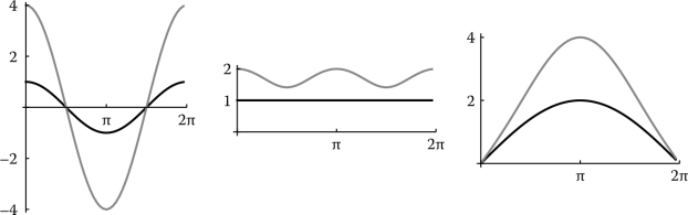
Inner product: comparing the dot product (black) with the test inner product from Example 14.9 (gray). For each plot, the unitvector r is rotated in the range [0, 2π]. Left: the graph of the inner products, e1 · r and ‹e1, r›. Middle: length for the inner products, and . Right: distance for the inner products, and
We will now show that this definition satisfies the inner product properties.
We can question the usefulness of this inner product, but it does satisfy the necessary properties.
Inner product spaces offer the concept of length,
This is also called the 2-norm or Euclidean norm and is denoted as ∥v∥2. Since the 2-norm is the most commonly used norm, the subscript is typically omitted. (More vector norms were introduced in Section 13.2.) Then the distance between two vectors,
For vectors in ℝn and the dot product, we have the Euclidean norm
and
Let’s get a feel for the norm and distance concept for the test inner product in (14.7). We have
The dot product produces ∥e1∥ = 1 and
Figure 14.3 illustrates the difference between the dot product and the test inner product. Again, r is a unit vector, rotated in the range [0, 2π]. The middle plot shows that unit length vectors with respect to the dot product are not unit length with respect to the test inner product. The right plot shows that the distance between two vectors differs too.
Orthogonality is important to establish as well. If two vectors v and w in a linear space satisfy
then they are called orthogonal. If v 1, ..., vn form a basis for and all vi are mutually orthogonal, (vi, vj) = 0 for i ≠ j, then the vi are said to form an orthogonal basis. If in addition they are also of unit length, , they form an orthonormal basis. Any basis of a linear space may be transformed to an orthonormal basis by the Gram-Schmidt process, described in Section 14.4.
The Cauchy-Schwartz inequality was introduced in (2.23) for ℝ2, and we repeat it here in the context of inner product spaces,
Equality holds if and only if v and w are linearly dependent.
If we restate the Cauchy-Schwartz inequality
and rearrange,
we obtain
Now we can express the angle θ between v and w by
The properties defining an inner product (14.3), (14.4), (14.5) and (14.6) suggest
A fourth property is the triangle inequality,
which we derived from the Cauchy-Schwartz inequality in Section 2.9.
See Sketch 2.22 for an illustration of this with respect to a triangle formed from two vectors in ℝ2. See the exercises for the generalized Pythagorean theorem.
The tools associated with the inner product are key for orthogonal decomposition and best approximation in a linear space. Recall that these concepts were introduced in Section 2.8 and have served as the building blocks for the 3D Gram-Schmidt method for construction of an orthonormal coordinate frame (Section 11.8) and least squares approximation (Section 12.7).
We finish with the general definition of a projection. Let u1, ..., uk span a subspace of . If v is a vector not in that space, then
is v’s orthogonal projection into .
14.4 Gram-Schmidt Orthonormalization
In Section 11.8 we built an orthonormal coordinate frame in ℝ3 using the Gram-Schmidt method. Every inner product space has an orthonormal basis. The key elements of its construction are projections and vector decomposition.
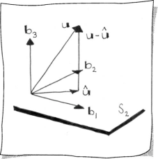
Let b1, ..., br be a set of orthonormal vectors, forming the basis of an r-dimensional subspace of , where n > r. We want to find br+1 orthogonal to the given bi. Let u be an arbitrary vector in , but not in . Define a vector by
This vector is u’s orthogonal projection into . To see this, we check that the difference vector is orthogonal to each of the bi. We first check that it is orthogonal to b1 and observe
All terms etc. vanish since the bi are mutually orthogonal and . Thus, . In the same manner, we show that is orthogonal to the remaining bi. Thus
Thus and the set b1, ..., br+1 forms an orthonormal basis for the subspace of . We may repeat this process until we have found an orthonormal basis for all of .
Sketch 14.1 provides an illustration in which is depicted as ℝ2. This process is known as Gram-Schmidt orthonormalization. Given any basis v1, ..., vn of , we can find an orthonormal basis by setting and continuing to construct, one by one, vectors b2, ..., bn using the above procedure. For instance,
Consult Section 11.8 for an example in ℝ3.
Suppose we are given the following vectors in ℝ4,
and we wish to form an orthonormal basis, b1, b2, b3, b4.
The Gram-Schmidt method, as defined in the displayed equations above, produces
The final vector, b4, is defined as
Knowing that the bi are normalized and checking that bi · bj = 0, we can be confident that this is an orthonormal basis. Another tool we have is the determinant, which will be one,
14.5 A Gallery of Spaces
In this section, we highlight some special linear spaces—but there are many more!
For a first example, consider all polynomials of a fixed degree n. These are functions of the form
where t is the independent variable of p(t). Thus we can construct a linear space Pn whose elements are all polynomials of a fixed degree. Addition in this space is addition of polynomials, i.e., coefficient by coefficient; multiplication is multiplication of a polynomial by a real number. It is easy to check that these polynomials have the linearity property (14.1). For example, if p(t) = 3 − 2t + 3t2 and q(t) = −1 + t + 2t2, then 2p(t) + 3q(t) = 3 − t + 12t2 is yet another polynomial of the same degree.
This example also serves to introduce a not-so-obvious linear map: the operation of forming derivatives! The derivative p′ of a degree n polynomial p is a polynomial of degree n − 1, given by
The linear map of forming derivatives thus maps the space of all degree n polynomials into that of all degree n − 1 polynomials. The rank of this map is thus n − 1.
Let us consider the two cubic polynomials
in the linear space of cubic polynomials, P3. Let
Now
It is now trivial to check that thus asserting the linearity of the derivative map.
For a second example, a linear space is given by the set of all realvalued continuous functions over the interval [0, 1]. This space is typically named C[0, 1]. Clearly the linearity condition is met: if f and g are elements of C[0, 1], then αf + βg is also in C[0, 1]. Here we have an example of a linear space that is infinite-dimensional, meaning that no finite set of functions forms a basis for C[0, 1].
For a third example, consider the set of all 3 × 3 matrices. They form a linear space; this space consists of matrices. In this space, linear combinations are formed using standard matrix addition and multiplication with a scalar as summarized in Section 9.11.
And, finally, a more abstract example. The set of all linear maps from a linear space into the reals forms a linear space itself and it is called the dual space of . As indicated by the notation, its dimension equals that of . The linear maps in are known as linear functionals.
For an example, let a fixed vector v and a variable vector u be in . The linear functionals defined by ΦV (u) = ‹u, v› are in . Then, for any basis b1, ..., bn of , we can define linear functionals
These functionals form a basis for .
In ℝ2, consider the fixed vector
Then ΦV (u) = (u, v) = u1 − 2u2 for all vectors u, where is the dot product
Pick e1, e2 for a basis in ℝ2. The associated linear functionals are
Any linear functional Φ can now be defined as
where r1 and r2 are scalars.

- linear space
- vector space
- dimension
- linear combination
- linearity property
- linearly independent
- subspace
- span
- linear map
- image
- preimage
- domain
- range
- rank
- full rank
- rank deficient
- inverse
- determinant
- inner product
- inner product space
- distance in an inner product space
- length in an inner product space
- orthogonal
- Gram-Schmidt method
- projection
- basis
- orthonormal
- orthogonal decomposition
- best approximation
- dual space
- linear functional
14.6 Exercises
Given elements of ℝ4,
is r = 3u + 6v + 2w also in ℝ4?
Given matrices that are elements of ,
is C = 4A + B an element of ?
- Does the set of all polynomials with an = 1 form a linear space?
- Does the set of all 3D vectors with nonnegative components form a subspace of ℝ3?
-
linearly independent?
Are
linearly independent?
Is the vector
in the subspace defined by u, v, w defined in Exercise 5?
Is the vector
in the subspace defined by u, v, w defined in Exercise 6?
- What is the dimension of the linear space formed by all n × n matrices?
Suppose we are given a linear map A : ℝ4 → ℝ2, preimage vectors vi, and corresponding image vectors wi. What are the dimensions of the matrix A ? The following linear relationship exists among the preimages,
What relationship holds for w4 with respect to the wi?
What is the rank of the matrix
What is the rank of the matrix
-
find , and dist(w, r) with respect to the dot product and then for the test inner product in (14.7).
For v, w in ℝ3, does
satisfy the requirements of an inner product?
For v, w in ℝ3, does
satisfy the requirements of an inner product?
In the space of all 3 × 3 matrices, is
an inner product?
Let p(t) = po + p1t + p2t2 and q(t) = q0 + q1t + q2t2 be two quadratic polynomials. Define
Is this an inner product for the space of all quadratic polynomials?
Show that the Pythagorean theorem
holds for orthogonal vectors v and w in an inner product space.
Given the following vectors in ℝ3,
form an orthonormal basis, b1, b2, b3.
Given the following vectors in ℝ4,
form an orthonormal basis, b1 = v1, b2, b3, b4.
- Find a basis for the linear space formed by all 2 × 2 matrices.
- Does the set of all monotonically increasing functions over [0, 1] form a linear space?
- Let be a linear space. Is the map Φ(u) = ∥u∥ an element of the dual space ?
- Show the linearity of the derivative map on the linear space of quadratic polynomials P2.
1Note that we will not always use the notation, but rather the standard name for the space when one exists.