A class diagram shows classes, their internal structures, and the static (compile-time) relationships among them. Figure B.1 shows the various presentation options for classes.

Figure B.1. Various levels of detail, visibility, and properties of classes.

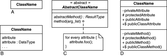
Figure B.2 shows the different presentation options for inheritance (the is-a-kind-of relationship). The generalization arrow always points from the subclass to the superclass. The right-hand side of Figure B.2 shows an inheritance tree that indicates an open-ended number of subclasses.

Figure B.2. Different presentation options for the generalization and specialization of classes.

Figure B.3 shows the aggregation of classes (the has-a-component relationship). An aggregation relationship implies that one object physically or conceptually contains another. The notation for aggregation consists of a line with a diamond at its base. The diamond is at the side of the owner class (whole class), and the line extends to the component class (part class). The full diamond represents physical containment; that is, the instance of the part class physically residing in the instance of the whole class (composite aggregation). A weaker form of aggregation, denoted with an empty diamond, indicates that the whole class has only a reference or pointer to the part instance but does not physically contain it. A name for the reference might appear at the base (e.g., part1 in Figure B.3). Aggregation also could indicate multiplicity and navigability between the whole and the parts.

Figure B.3. Aggregation, navigability, and multiplicity.

Figure B.4 shows a collaboration of classes as a dashed ellipse containing the name of the collaboration (stereotyped here as a pattern). The dashed lines emanating from the collaboration symbol to the various elements denote participants in the collaboration. Each line is labeled by the role that the participant plays in the collaboration. The roles correspond to the names of elements within the context for the collaboration; such names in the collaboration are treated as parameters that are bound to specific elements on each occurrence of the pattern within a model [OMG 07].

Figure B.4. Design pattern as a collaboration of classes

A state diagram shows the static state space of a given context class, the events that cause a transition from one state to another, and the actions that result.

Figure B.5 shows the presentation options for states and the notation for a state transition. A state is always denoted by a rectangle with rounded corners. The name of the state appears in bold type at the top. Optionally, right below the name, a state can have an internal transition compartment separated from the name by a horizontal line. The internal transition compartment can contain entry actions (actions following the reserved symbol entry), exit actions (actions following the reserved symbol exit), and other internal transitions (e.g., those triggered by EVT in Figure B.5).

Figure B.5. States and a transition.

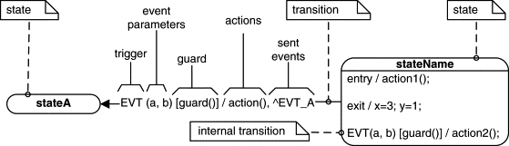
A state transition is represented as an arrow originating at the boundary of the source state and pointing to the boundary of the target state. At a minimum, a transition must be labeled with the triggering event. Optionally, the trigger can be followed by event parameters, a guard, a list of actions, and a list of events that have been sent.

Figure B.6 shows a composite state (superstate) that contains other states (substates). Each composite state can have a separate initial transition to designate the initial substate. Although Figure B.6 shows only one level of nesting, the substates can be composite as well.

Figure B.6. Composite state, initial transitions, and the final state.

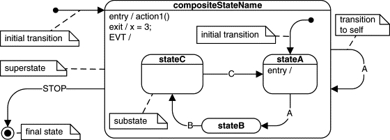
Figure B.7 shows composite “stateA” with the orthogonal regions (AND-states) separated by a dashed line and two pseudostates: the choicepoint and the deep history.

Figure B.7. Orthogonal regions and pseudostates.

A sequence diagram shows a particular sequence of event instances exchanged among objects at runtime. A sequence diagram has two dimensions; the vertical dimension represents time and the horizontal dimension represents different objects. Time flows down the page (the dimensions can be reversed, if desired).

Figure B.8 shows an example of a sequence diagram. Object boxes, together with the descending vertical lines, represent objects participating in the scenario. As always in the UML specification, the object name in each box is underlined (some objects may be identified only by a colon and a class name). Heavy borders indicate active objects.

Figure B.8. Sequence diagram.

Events are represented as horizontal arrows originating from the sending object and terminating at the receiving object. Optionally, thin rectangles around instance lines can indicate focus of control. Sequence diagrams also can contain state marks to indicate explicit state changes resulting from the event exchange.

A timing diagram shows the explicit changes of state in one or more objects along a single time axis. Figure B.9 shows an example of a timing diagram for multiple objects (T1, T2, and T3). The timing diagram has two dimensions; time flows along the horizontal axis and the object state along the vertical axis. Each object is assigned a horizontal band across the diagram (a “swim lane”) separated from other bands by dashed lines. Presentation options include deadlines, propagated events, and jitter.

Figure B.9. Timing diagram.