A state captures the relevant aspects of the system's history very efficiently. For example, when you strike a key on a keyboard, the character code generated will be either an uppercase or a lowercase character, depending on whether the Caps Lock is active.² Ignore at this print the effects of the Shift, Ctrl, and Alt keys. Therefore, the keyboard's behavior can be divided into two chunks (states): the “default” state and the “caps_locked” state. (Most keyboards actually have an LED that indicates that the keyboard is in the “caps_locked” state.) The behavior of a keyboard depends only on certain aspects of its history, namely whether the Caps Lock key has been pressed, but not, for example, on how many and exactly which other keys have been pressed previously. A state can abstract away all possible (but irrelevant) event sequences and capture only the relevant ones.

To relate this concept to programming, this means that instead of recording the event history in a multitude of variables, flags, and convoluted logic, you rely mainly on just one state variable that can assume only a limited number of a priori determined values (e.g., two values in case of the keyboard). The value of the state variable crisply defines the current state of the system at any given time. The concept of state reduces the problem of identifying the execution context in the code to testing just the state variable instead of many variables, thus eliminating a lot of conditional logic. Actually, in all but the most basic state machine implementation techniques, such as the “nested-switch statement” technique discussed in Chapter 3, even the explicit testing of the state variable disappears from the code, which reduces the “spaghetti” further still (you will experience this effect later in Chapters 3 and 4). Moreover, switching between different states is vastly simplified as well, because you need to reassign just one state variable instead of changing multiple variables in a self-consistent manner.

FSMs have an expressive graphical representation in the form of state diagrams. These diagrams are directed graphs in which nodes denote states and connectors denote state transitions.³ Appendix B contains a succinct summary of the graphical notations used throughout the book, including state transition diagrams.

For example, Figure 2.2 shows a UML state transition diagram corresponding to the computer keyboard state machine. In UML, states are represented as rounded rectangles labeled with state names. The transitions, represented as arrows, are labeled with the triggering events followed optionally by the list of executed actions. The initial transition originates from the solid circle and specifies the starting state when the system first begins. Every state diagram should have such a transition, which should not be labeled, since it is not triggered by an event. The initial transition can have associated actions.

Figure 2.2. UML state diagram representing the computer keyboard state machine.

Newcomers to the state machine formalism often confuse state diagrams with flowcharts. The UML specification [OMG 07] isn't helping in this respect because it lumps activity graphs in the state machine package. Activity graphs are essentially elaborate flowcharts.

Figure 2.3 shows a comparison of a state diagram with a flowchart. A state machine (panel (A)) performs actions in response to explicit triggers. In contrast, the flowchart (panel (B)) does not need explicit triggers but rather transitions from node to node in its graph automatically upon completion of activities.

Figure 2.3. Comparison of (A) state machine (statechart) with (B) activity diagram (flowchart).

Graphically, compared to state diagrams, flowcharts reverse the sense of vertices and arcs. In a state diagram, the processing is associated with the arcs (transitions), whereas in a flowchart, it is associated with the vertices. A state machine is idle when it sits in a state waiting for an event to occur. A flowchart is busy executing activities when it sits in a node. Figure 2.3 attempts to show that reversal of roles by aligning the arcs of the statecharts with the processing stages of the flowchart.

You can compare a flowchart to an assembly line in manufacturing because the flowchart describes the progression of some task from beginning to end (e.g., transforming source code input into object code output by a compiler). A state machine generally has no notion of such a progression. A computer keyboard, for example, is not in a more advanced stage when it is in the “caps_locked” state, compared to being in the “default” state; it simply reacts differently to events. A state in a state machine is an efficient way of specifying a particular behavior, rather than a stage of processing.

The distinction between state machines and flowcharts is especially important because these two concepts represent two diametrically opposed programming paradigms: event-driven programming (state machines) and transformational programming (flowcharts). You cannot devise effective state machines without constantly thinking about the available events. In contrast, events are only a secondary concern (if at all) for flowcharts.

One possible interpretation of state for software systems is that each state represents one distinct set of valid values of the whole program memory. Even for simple programs with only a few elementary variables, this interpretation leads to an astronomical number of states. For example, a single 32-bit integer could contribute to over 4 billion different states. Clearly, this interpretation is not practical, so program variables are commonly dissociated from states. Rather, the complete condition of the system (called the extended state) is the combination of a qualitative aspect (the state) and the quantitative aspects (the extended state variables). In this interpretation, a change of variable does not always imply a change of the qualitative aspects of the system behavior and therefore does not lead to a change of state [Selic+ 94].

State machines supplemented with variables are called extended state machines. Extended state machines can apply the underlying formalism to much more complex problems than is practical without including extended state variables. For instance, suppose the behavior of the keyboard depends on the number of characters typed on it so far and that after, say, 1,000 keystrokes, the keyboard breaks down and enters the final state. To model this behavior in a state machine without memory, you would need to introduce 1,000 states (e.g., pressing a key in state stroke123 would lead to state stroke124, and so on), which is clearly an impractical proposition. Alternatively, you could construct an extended state machine with a key_count down-counter variable. The counter would be initialized to 1,000 and decremented by every keystroke without changing state. When the counter reached zero, the state machine would enter the final state.

The state diagram from Figure 2.4 is an example of an extended state machine, in which the complete condition of the system (called the extended state) is the combination of a qualitative aspect—the “state”—and the quantitative aspects—the extended state variables (such as the down-counter key_count). In extended state machines, a change of a variable does not always imply a change of the qualitative aspects of the system behavior and therefore does not always lead to a change of state.

Figure 2.4. Extended state machine of “cheap keyboard” with extended state variable key_count and various guard conditions.

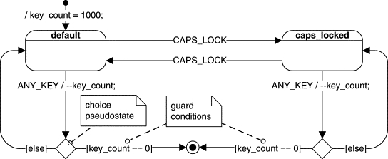
The obvious advantage of extended state machines is flexibility. For example, extending the lifespan of the “cheap keyboard” from 1,000 to 10,000 keystrokes would not complicate the extended state machine at all. The only modification required would be changing the initialization value of the key_count down-counter in the initial transition.

This flexibility of extended state machines comes with a price, however, because of the complex coupling between the “qualitative” and the “quantitative” aspects of the extended state. The coupling occurs through the guard conditions attached to transitions, as shown in Figure 2.4.

Guard conditions (or simply guards) are Boolean expressions evaluated dynamically based on the value of extended state variables and event parameters (see the discussion of events and event parameters in the next section). Guard conditions affect the behavior of a state machine by enabling actions or transitions only when they evaluate to TRUE and disabling them when they evaluate to FALSE. In the UML notation, guard conditions are shown in square brackets (e.g., [key_count == 0]).

The need for guards is the immediate consequence of adding memory (extended state variables) to the state machine formalism. Used sparingly, extended state variables and guards make up an incredibly powerful mechanism that can immensely simplify designs. But don't let the fancy name (“guard”) and the concise UML notation fool you. When you actually code an extended state machine, the guards become the same IFs and ELSEs that you wanted to eliminate by using the state machine in the first place. Too many of them, and you'll find yourself back in square one (“spaghetti”), where the guards effectively take over handling of all the relevant conditions in the system.

Indeed, abuse of extended state variables and guards is the primary mechanism of architectural decay in designs based on state machines. Usually, in the day-to-day battle, it seems very tempting, especially to programmers new to state machine formalism, to add yet another extended state variable and yet another guard condition (another if or an else) rather than to factor out the related behavior into a new qualitative aspect of the system—the state. From my experience in the trenches, the likelihood of such an architectural decay is directly proportional to the overhead (actual or perceived) involved in adding or removing states. (That's why I don't particularly like the popular state-table technique of implementing state machines that I describe in Chapter 3, because adding a new state requires adding and initializing a whole new column in the table.)

One of the main challenges in becoming an effective state machine designer is to develop a sense for which parts of the behavior should be captured as the “qualitative” aspects (the “state”) and which elements are better left as the “quantitative” aspects (extended state variables). In general, you should actively look for opportunities to capture the event history (what happened) as the “state” of the system, instead of storing this information in extended state variables. For example, the Visual Basic calculator uses an extended state variable DecimalFlag to remember that the user entered the decimal point to avoid entering multiple decimal points in the same number. However, a better solution is to observe that entering a decimal point really leads to a distinct state “entering_the_fractional_part_of_a_number,” in which the calculator ignores decimal points. This solution is superior for a number of reasons. The lesser reason is that it eliminates one extended state variable and the need to initialize and test it. The more important reason is that the state-based solution is more robust because the context information is used very locally (only in this particular state) and is discarded as soon as it becomes irrelevant. Once the number is correctly entered, it doesn't really matter for the subsequent operation of the calculator whether that number had a decimal point. The state machine moves on to another state and automatically “forgets” the previous context. The DecimalFlag extended state variable, on the other hand, “lays around” well past the time the information becomes irrelevant (and perhaps outdated!). Worse, you must not forget to reset DecimalFlag before entering another number or the flag will incorrectly indicate that indeed the user once entered the decimal point, but perhaps this happened in the context of the previous number.

Capturing behavior as the quantitative “state” has its disadvantages and limitations, too. First, the state and transition topology in a state machine must be static and fixed at compile time, which can be too limiting and inflexible. Sure, you can easily devise “state machines” that would modify themselves at runtime (this is what often actually happens when you try to recode “spaghetti” as a state machine). However, this is like writing self-modifying code, which indeed was done in the early days of programming but was quickly dismissed as a generally bad idea. Consequently, “state” can capture only static aspects of the behavior that are known a priori and are unlikely to change in the future.

For example, it's fine to capture the entry of a decimal point in the calculator as a separate state “entering_the_fractional_part_of_a_number,” because a number can have only one fractional part, which is both known a priori and is not likely to change in the future. However, implementing the “cheap keyboard” without extended state variables and guard conditions would be practically impossible. This example points to the main weakness of the quantitative “state,” which simply cannot store too much information (such as the wide range of keystroke counts). Extended state variables and guards are thus a mechanism for adding extra runtime flexibility to state machines.

In the most general terms, an event is an occurrence in time and space that has significance to the system. Strictly speaking, in the UML specification the term event refers to the type of occurrence rather than to any concrete instance of that occurrence [OMG 07]. For example, Keystroke is an event for the keyboard, but each press of a key is not an event but a concrete instance of the Keystroke event. Another event of interest for the keyboard might be Power-on, but turning the power on tomorrow at 10:05:36 will be just an instance of the Power-on event.

An event can have associated parameters, allowing the event instance to convey not only the occurrence of some interesting incident but also quantitative information regarding that occurrence. For example, the Keystroke event generated by pressing a key on a computer keyboard has associated parameters that convey the character scan code as well as the status of the Shift, Ctrl, and Alt keys.

An event instance outlives the instantaneous occurrence that generated it and might convey this occurrence to one or more state machines. Once generated, the event instance goes through a processing life cycle that can consist of up to three stages. First, the event instance is received when it is accepted and waiting for processing (e.g., it is placed on the event queue). Later, the event instance is dispatched to the state machine, at which point it becomes the current event. Finally, it is consumed when the state machine finishes processing the event instance. A consumed event instance is no longer available for processing.

When an event instance is dispatched, the state machine responds by performing actions, such as changing a variable, performing I/O, invoking a function, generating another event instance, or changing to another state. Any parameter values associated with the current event are available to all actions directly caused by that event.

Switching from one state to another is called state transition, and the event that causes it is called the triggering event, or simply the trigger. In the keyboard example, if the keyboard is in the “default” state when the Caps Lock key is pressed, the keyboard will enter the “caps_locked” state. However, if the keyboard is already in the “caps_locked” state, pressing Caps Lock will cause a different transition—from the “caps_locked” to the “default” state. In both cases, pressing Caps Lock is the triggering event.

In extended state machines, a transition can have a guard, which means that the transition can “fire” only if the guard evaluates to TRUE. A state can have many transitions in response to the same trigger, as long as they have nonoverlapping guards; however, this situation could create problems in the sequence of evaluation of the guards when the common trigger occurs. The UML specification intentionally does not stipulate any particular order; rather, UML puts the burden on the designer to devise guards in such a way that the order of their evaluation does not matter. Practically, this means that guard expressions should have no side effects, at least none that would alter evaluation of other guards having the same trigger.

All state machine formalisms, including UML statecharts, universally assume that a state machine completes processing of each event before it can start processing the next event. This model of execution is called run to completion, or RTC.

In the RTC model, the system processes events in discrete, indivisible RTC steps. New incoming events cannot interrupt the processing of the current event and must be stored (typically in an event queue) until the state machine becomes idle again. These semantics completely avoid any internal concurrency issues within a single state machine. The RTC model also gets around the conceptual problem of processing actions associated with transitions,⁴ State machines that associate actions with transitions are classified as Mealy machines. where the state machine is not in a well-defined state (is between two states) for the duration of the action. During event processing, the system is unresponsive (unobservable), so the ill-defined state during that time has no practical significance.

Note, however, that RTC does not mean that a state machine has to monopolize the CPU until the RTC step is complete. The preemption restriction only applies to the task context of the state machine that is already busy processing events. In a multitasking environment, other tasks (not related to the task context of the busy state machine) can be running, possibly preempting the currently executing state machine. As long as other state machines do not share variables or other resources with each other, there are no concurrency hazards.

The key advantage of RTC processing is simplicity. Its biggest disadvantage is that the responsiveness of a state machine is determined by its longest RTC step.⁵ A state machine can improve responsiveness by breaking up the CPU-intensive processing into sufficiently short RTC steps (see also the “Reminder” state pattern in Chapter 5). Achieving short RTC steps can often significantly complicate real-time designs.

All reactive systems seem to reuse behavior in a similar way. For example, the characteristic look and feel of all GUIs results from the same pattern, which the Windows guru Charles Petzold calls the “Ultimate Hook” [Petzold 96]. The pattern is brilliantly simple: A GUI system dispatches every event first to the application (e.g., Windows calls a specific function inside the application, passing the event as an argument). If not handled by the application, the event flows back to the system. This establishes a hierarchical order of event processing. The application, which is conceptually at a lower level of the hierarchy, has the first shot at every event; thus the application can choose to react in any way it likes. At the same time, all unhandled events flow back to the higher level (i.e., to the GUI system), where they are processed according to the standard look and feel. This is an example of programming by difference because the application programmer needs to code only the differences from the standard system behavior.

Harel statecharts bring the “Ultimate Hook” pattern to the logical conclusion by combining it with the state machine formalism. The most important innovation of statecharts over the classical FSMs is the introduction of hierarchically nested states (that's why statecharts are also called hierarchical state machines, or HSMs). The semantics associated with state nesting are as follows (see Figure 2.5(A)): If a system is in the nested state “s11” (called the substate), it also (implicitly) is in the surrounding state “s1” (called the superstate). This state machine will attempt to handle any event in the context of state “s11,” which conceptually is at the lower level of the hierarchy. However, if state “s11” does not prescribe how to handle the event, the event is not quietly discarded as in a traditional “flat” state machine; rather, it is automatically handled at the higher level context of the superstate “s1.” This is what is meant by the system being in state “s11” as well as “s1.” Of course, state nesting is not limited to one level only, and the simple rule of event processing applies recursively to any level of nesting.

Figure 2.5. UML notation for hierarchically nested states (A), and a state model of a toaster oven in which states “toasting” and “baking” share the common transition from state “heating” to “door_open” (B).

States that contain other states are called composite states; conversely, states without internal structure are called simple states or leaf states. A nested state is called a direct substate when it is not contained by any other state; otherwise, it is referred to as a transitively nested substate.

Because the internal structure of a composite state can be arbitrarily complex, any hierarchical state machine can be viewed as an internal structure of some (higher-level) composite state. It is conceptually convenient to define one composite state as the ultimate root of state machine hierarchy. In the UML specification, every state machine has a top state (the abstract root of every state machine hierarchy), which contains all the other elements of the entire state machine. The graphical rendering of this all-enclosing top state is optional [OMG 07].

As you can see, the semantics of hierarchical state decomposition are designed to facilitate sharing of behavior through the direct support for the “Ultimate Hook” pattern. The substates (nested states) need only define the differences from the superstates (surrounding states). A substate can easily reuse the common behavior from its superstate(s) by simply ignoring commonly handled events, which are then automatically handled by higher-level states. In this manner, the substates can share all aspects of behavior with their superstates. For example, in a state model of a toaster oven shown in Figure 2.5(B), states “toasting” and “baking” share a common transition DOOR_OPEN to the “door_open” state, defined in their common superstate “hating.”

The aspect of state hierarchy emphasized most often is abstraction—an old and powerful technique for coping with complexity. Instead of facing all aspects of a complex system at the same time, it is often possible to ignore (abstract away) some parts of the system. Hierarchical states are an ideal mechanism for hiding internal details because the designer can easily zoom out or zoom in to hide or show nested states. Although abstraction by itself does not reduce overall system complexity, it is valuable because it reduces the amount of detail you need to deal with at one time. As Grady Booch [Booch 94] notes:

However valuable abstraction in itself might be, you cannot cheat your way out of complexity simply by hiding it inside composite states. However, the composite states don't simply hide complexity, they also actively reduce it through the powerful mechanism of reuse (the “Ultimate Hook” pattern). Without such reuse, even a moderate increase in system complexity often leads to an explosive increase in the number of states and transitions. For example, if you transform the statechart from Figure 2.5(B) to a classical flat state machine,⁶ Such a transformation is always possible because HSMs are mathematically equivalent to classical FSMs. you must repeat one transition (from heating to “door_open”) in two places: as a transition from “toasting” to “door_open” and from “baking” to “door_open.” Avoiding such repetitions allows HSMs to grow proportionally to system complexity. As the modeled system grows, the opportunity for reuse also increases and thus counteracts the explosive increase in states and transitions typical for traditional FSMs.

Hierarchical states are more than merely the “grouping of [nested] state machines together without additional semantics” [Mellor 00]. In fact, hierarchical states have simple but profound semantics. Nested states are also more than just “great diagrammatic simplification when a set of events applies to several substates” [Douglass 99]. The savings in the number of states and transitions are real and go far beyond less cluttered diagrams. In other words, simpler diagrams are just a side effect of behavioral reuse enabled by state nesting.

The fundamental character of state nesting comes from the combination of abstraction and hierarchy, which is a traditional approach to reducing complexity and is otherwise known in software as inheritance. In OOP, the concept of class inheritance describes relations between classes of objects. Class inheritance describes the “is a …” relationship among classes. For example, class Bird might derive from class Animal. If an object is a bird (instance of the Bird class), it automatically is an animal, because all operations that apply to animals (e.g., eating, eliminating, reproducing) also apply to birds. But birds are more specialized, since they have operations that are not applicable to animals in general. For example, flying() applies to birds but not to fish.

The benefits of class inheritance are concisely summarized by Gamma and colleagues [Gamma+ 95]:

As you saw in the previous section, all these basic characteristics of inheritance apply equally well to nested states (just replace the word class with state), which is not surprising because state nesting is based on the same fundamental “is a …” classification as object-oriented class inheritance. For example, in a state model of a toaster oven, state “toasting” nests inside state “heating.” If the toaster is in the “toasting” state, it automatically is in the “heating” state because all behavior pertaining to “heating” applies also to “toasting” (e.g., the heater must be turned on). But “toasting” is more specialized because it has behaviors not applicable to “heating” in general. For example, setting toast color (light or dark) applies to “toasting” but not to “baking.”

In the case of nested states, the “is a …” (is-a-kind-of) relationship merely needs to be replaced by the “is in …” (is-in-a-state) relationship; otherwise, it is the same fundamental classification. State nesting allows a substate to inherit state behavior from its ancestors (superstates); therefore, it's called behavioral inheritance.

The concept of inheritance is fundamental in software construction. Class inheritance is essential for better software organization and for code reuse, which makes it a cornerstone of OOP. In the same way, behavioral inheritance is essential for efficient use of HSMs and for behavior reuse, which makes it a cornerstone of event-driven programming. In Chapter 5, a mini-catalog of state patterns shows ways to structure HSMs to solve recurring problems. Not surprisingly, behavioral inheritance plays the central role in all these patterns.

Identifying the relationship among substates and superstates as inheritance has many practical implications. Perhaps the most important is the Liskov Substitution Principle (LSP) applied to state hierarchy. In its traditional formulation for classes, LSP requires that a subclass can be freely substituted for its superclass. This means that every instance of the subclass should be compatible with the instance of the superclass and that any code designed to work with the instance of the superclass should continue to work correctly if an instance of the subclass is used instead.

Because behavioral inheritance is just a special kind of inheritance, LSP can be applied to nested states as well as classes. LSP generalized for states means that the behavior of a substate should be consistent with the superstate. For example, all states nested inside the “heating” state of the toaster oven (e.g., “toasting” or “baking”) should share the same basic characteristics of the “heating” state. In particular, if being in the “heating” state means that the heater is turned on, then none of the substates should turn the heater off (without transitioning out of the “heating” state). Turning the heater off and staying in the “toasting” or “baking” state would be inconsistent with being in the “heating” state and would indicate poor design (violation of the LSP).

Compliance with the LSP allows you to build better (more correct) state hierarchies and make efficient use of abstraction. For example, in an LSP-compliant state hierarchy, you can safely zoom out and work at the higher level of the “heating” state (thus abstracting away the specifics of “toasting” and “baking”). As long as all the substates are consistent with their superstate, such abstraction is meaningful. On the other hand, if the substates violate basic assumptions of being in the superstate, zooming out and ignoring the specifics of the substates will be incorrect.

Hierarchical state decomposition can be viewed as exclusive-OR operation applied to states. For example, if a system is in the “heating” superstate (Figure 2.5(B)), it means that it's either in “toasting” substate OR the “baking” substate. That is why the “heating” superstate is called an OR-state.

UML statecharts also introduce the complementary AND-decomposition. Such decomposition means that a composite state can contain two or more orthogonal regions (orthogonal means independent in this context) and that being in such a composite state entails being in all its orthogonal regions simultaneously [Harel+ 98].

Orthogonal regions address the frequent problem of a combinatorial increase in the number of states when the behavior of a system is fragmented into independent, concurrently active parts. For example, apart from the main keypad, a computer keyboard has an independent numeric keypad. From the previous discussion, recall the two states of the main keypad already identified: “default” and “caps_locked” (Figure 2.2). The numeric keypad also can be in two states—“numbers” and “arrows”—depending on whether Num Lock is active. The complete state space of the keyboard in the standard decomposition is the cross-product of the two components (main keypad and numeric keypad) and consists of four states: “default–numbers,” “default–arrows,” “caps_locked–numbers,” and “caps_locked–arrows.” However, this is unnatural because the behavior of the numeric keypad does not depend on the state of the main keypad and vice versa. Orthogonal regions allow you to avoid mixing the independent behaviors as a cross-product and, instead, to keep them separate, as shown in Figure 2.6.

Figure 2.6. Two orthogonal regions (main keypad and numeric keypad) of a computer keyboard.

Note that if the orthogonal regions are fully independent of each other, their combined complexity is simply additive, which means that the number of independent states needed to model the system is simply the sum k + l + m + …, where k, l, m, … denote numbers of OR-states in each orthogonal region. The general case of mutual dependency, on the other hand, results in multiplicative complexity, so in general, the number of states needed is the product k × l × m × ….

In most real-life situations, however, orthogonal regions are only approximately orthogonal (i.e., they are not independent). Therefore, UML statecharts provide a number of ways for orthogonal regions to communicate and synchronize their behaviors. From these rich sets of (sometimes complex) mechanisms, perhaps the most important is that orthogonal regions can coordinate their behaviors by sending event instances to each other.

Even though orthogonal regions imply independence of execution (i.e., some kind of concurrency), the UML specification does not require that a separate thread of execution be assigned to each orthogonal region (although it can be implemented that way). In fact, most commonly, orthogonal regions execute within the same thread. The UML specification only requires that the designer not rely on any particular order in which an event instance will be dispatched to the involved orthogonal regions.

Every state in a UML statechart can have optional entry actions, which are executed upon entry to a state, as well as optional exit actions, which are executed upon exit from a state. Entry and exit actions are associated with states, not transitions.⁷ State machines are classified as Mealy machines if actions are associated with transitions and as Moore machines if actions are associated with states. UML state machines have characteristics of both Mealy machines and Moore machines. Regardless of how a state is entered or exited, all its entry and exit actions will be executed. Because of this characteristic, statecharts behave like Moore automata. The UML notation for state entry and exit actions is to place the reserved word “entry” (or “exit”) in the state right below the name compartment, followed by the forward slash and the list of arbitrary actions (see Figure 2.7).

Figure 2.7. Toaster oven state machine with entry and exit actions.

The value of entry and exit actions is that they provide means for guaranteed initialization and cleanup, very much like class constructors and destructors in OOP. For example, consider the “door_open” state from Figure 2.7, which corresponds to the toaster oven behavior while the door is open. This state has a very important safety-critical requirement: Always disable the heater when the door is open.⁸ Commonly, such a safety-critical function is (and should be) redundantly safeguarded by mechanical interlocks, but for the sake of this discussion, suppose you need to implement it entirely in software. Additionally, while the door is open, the internal lamp illuminating the oven should light up.

Of course, you could model such behavior by adding appropriate actions (disabling the heater and turning on the light) to every transition path leading to the “door_open” state (the user may open the door at any time during “baking” or “toasting” or when the oven is not used at all). You also should not forget to extinguish the internal lamp with every transition leaving the “door_open” state. However, such a solution would cause the repetition of actions in many transitions. More important, such an approach is error-prone in view of changes to the state machine (e.g., the next programmer working on a new feature, such as top-browning, might simply forget to disable the heater on transition to “door_open”).

Entry and exit actions allow you to implement the desired behavior in a much safer, simpler, and more intuitive way. As shown in Figure 2.7, you could specify that the exit action from “heating” disables the heater, the entry action to “door_open” lights up the oven lamp, and the exit action from “door_open” extinguishes the lamp. The use of entry and exit action is superior to placing actions on transitions because it avoids repetitions of those actions on transitions and eliminates the basic safety hazard of leaving the heater on while the door is open. The semantics of exit actions guarantees that, regardless of the transition path, the heater will be disabled when the toaster is not in the “heating” state.

Figure 2.8. UML state diagram of the keyboard state machine with internal transitions.

Because entry actions are executed automatically whenever an associated state is entered, they often determine the conditions of operation or the identity of the state, very much as a class constructor determines the identity of the object being constructed. For example, the identity of the “heating” state is determined by the fact that the heater is turned on. This condition must be established before entering any substate of “heating” because entry actions to a substate of “heating,” like “toasting,” rely on proper initialization of the “heating” superstate and perform only the differences from this initialization. Consequently, the order of execution of entry actions must always proceed from the outermost state to the innermost state.

Not surprisingly, this order is analogous to the order in which class constructors are invoked. Construction of a class always starts at the very root of the class hierarchy and follows through all inheritance levels down to the class being instantiated. The execution of exit actions, which corresponds to destructor invocation, proceeds in the exact reverse order, starting from the innermost state (corresponding to the most derived class).

Very commonly, an event causes only some internal actions to execute but does not lead to a change of state (state transition). In this case, all actions executed comprise the internal transition. For example, when you type on your keyboard, it responds by generating different character codes. However, unless you hit the Caps Lock key, the state of the keyboard does not change (no state transition occurs). In UML, this situation should be modeled with internal transitions, as shown in Figure 2.8. The UML notation for internal transitions follows the general syntax used for exit (or entry) actions, except instead of the word entry (or exit) the internal transition is labeled with the triggering event (e.g., see the internal transition triggered by the ANY_KEY event in Figure 2.8).

In the absence of entry and exit actions, internal transitions would be identical to self-transitions (transitions in which the target state is the same as the source state). In fact, in a classical Mealy automaton, actions are associated exclusively with state transitions, so the only way to execute actions without changing state is through a self-transition (depicted as a directed loop in Figure 2.2). However, in the presence of entry and exit actions, as in UML statecharts, a self-transition involves the execution of exit and entry actions and therefore it is distinctively different from an internal transition.

In contrast to a self-transition, no entry or exit actions are ever executed as a result of an internal transition, even if the internal transition is inherited from a higher level of the hierarchy than the currently active state. Internal transitions inherited from superstates at any level of nesting act as if they were defined directly in the currently active state.

State nesting combined with entry and exit actions significantly complicates the state transition semantics in HSMs compared to the traditional FSMs. When dealing with hierarchically nested states and orthogonal regions, the simple term current state can be quite confusing. In an HSM, more than one state can be active at once. If the state machine is in a leaf state that is contained in a composite state (which is possibly contained in a higher-level composite state, and so on), all the composite states that either directly or transitively contain the leaf state are also active. Furthermore, because some of the composite states in this hierarchy might have orthogonal regions, the current active state is actually represented by a tree of states starting with the single top state at the root down to individual simple states at the leaves. The UML specification refers to such a state tree as state configuration [OMG 07].

In UML, a state transition can directly connect any two states. These two states, which may be composite, are designated as the main source and the main target of a transition. Figure 2.9 shows a simple transition example and explains the state roles in that transition. The UML specification prescribes that taking a state transition involves executing the following actions in the following sequence [OMG 07, Section 15.3.13]:

Figure 2.9. State roles in a state transition.

The transition sequence is easy to interpret in the simple case of both the main source and the main target nesting at the same level. For example, transition T1 shown in Figure 2.9 causes the evaluation of the guard g(); followed by the sequence of actions: a(); b(); t(); c(); d(); and e(), assuming that the guard g() evaluates to TRUE.

However, in the general case of source and target states nested at different levels of the state hierarchy, it might not be immediately obvious how many levels of nesting need to be exited. The UML specification prescribes that a transition involves exiting all nested states from the current active state (which might be a direct or transitive substate of the main source state) up to, but not including, the least common ancestor (LCA) state of the main source and main target states. As the name indicates, the LCA is the lowest composite state that is simultaneously a superstate (ancestor) of both the source and the target states. As described before, the order of execution of exit actions is always from the most deeply nested state (the current active state) up the hierarchy to the LCA but without exiting the LCA. For instance, the LCA(s1, s2) of states “s1” and “s2” shown in Figure 2.9 is state “s.”

Entering the target state configuration commences from the level where the exit actions left off (i.e., from inside the LCA). As described before, entry actions must be executed starting from the highest-level state down the state hierarchy to the main target state. If the main target state is composite, the UML semantics prescribes to “drill” into its submachine recursively using the local initial transitions. The target state configuration is completely entered only after encountering a leaf state that has no initial transitions.

One big problem with the UML transition sequence is that it requires executing actions associated with the transition after destroying the source state configuration but before creating the target state configuration. In the analogy between exit actions in state machines and destructors in OOP, this situation corresponds to executing a class method after partially destroying an object. Of course, such action is illegal in OOP. As it turns out, it is also particularly awkward to implement for state machines.

Executing actions associated with a transition is much more natural in the context of the source state—the same context in which the guard condition is evaluated. Only after the guard and the transition actions execute, the source state configuration is exited and the target state configuration is entered atomically. That way the state machine is observable only in a stable state configuration, either before or after the transition, but not in the middle.

Before UML 2, the only transition semantics in use was the external transition, in which the main source of the transition is always exited and the main target of the transition is always entered. UML 2 preserved the “external transition” semantics for backward compatibility, but also introduced a new kind of transition called local transition [OMG 07, Section 15.3.15]. For many transition topologies, external and local transitions are actually identical. However, a local transition doesn't cause exit from the main source state if the main target state is a substate of the main source. In addition, local state transition doesn't cause exit and reentry to the target state if the main target is a superstate of the main source state.

Figure 2.10 contrasts local (A) and external (B) transitions. In the top row, you see the case of the main source containing the target. The local transition does not cause exit from the source, while the external transition causes exit and re-entry to the source. In the bottom row of Figure 2.10, you see the case of the target containing the source. The local transition does not cause entry to the target, whereas the external transition causes exit and reentry to the target.

Figure 2.10. Local (A) versus external transitions (B). QP implements only the local transitions.

The UML specification defines four kinds of events, each one distinguished by a specific notation.

A SignalEvent is by far the most common event type (and the only one used in classical FSMs). Even here, however, the UML specification extends traditional FSM semantics by allowing the specified signal to be a subclass of another signal, resulting in polymorphic event triggering. Any transition triggered by a given signal event is also triggered by any subevent derived directly or indirectly from the original event.

Sometimes an event arrives at a particularly inconvenient time, when a state machine is in a state that cannot handle the event. In many cases, the nature of the event is such that it can be postponed (within limits) until the system enters another state, in which it is much better prepared to handle the original event.

UML state machines provide a special mechanism for deferring events in states. In every state, you can include a clause ‘deferred / [event list]’. If an event in the current state's deferred event list occurs, the event will be saved (deferred) for future processing until a state is entered that does not list the event in its deferred event list. Upon entry to such state, the UML state machine will automatically recall any saved event(s) that are no longer deferred and process them as if they have just arrived.

Because statecharts started as a visual formalism [Harel 87], some nodes in the diagrams other than the regular states turned out to be useful for implementing various features (or simply as a shorthand notation). The various “plumbing gear” nodes are collectively called pseudostates. More formally, a pseudostate is an abstraction that encompasses different types of transient vertices (nodes) in the state machine graph. The UML specification [OMG 07] defines the following kinds of pseudostates:

UML statecharts provide sufficiently well-defined semantics for building executable state models. Indeed, several design automation tools on the market support various versions of statecharts (see the sidebar “Design Automation Tools Supporting Statecharts”). The commercially available design automation tools typically not only automatically generate code from statecharts but also enable debugging and testing of the state models at the graphical level [Douglass 99].

But what does automatic code generation really mean? And more important, what kind of code is actually generated by such statechart-based tools?

Many people understand automatic code synthesis as the generation of a program to solve a problem from a statement of the problem specification. Statechart-based tools cannot provide this because a statechart is just a higher-level (mostly visual) solution rather than the statement of the problem.

As far as the automatically generated code is concerned, the statechart-based tools can autonomously generate only so-called “housekeeping code” [Douglass 99]. The modeler explicitly must provide all the application-specific code, such as action and guard expressions, to the tool. The role of housekeeping code is to “glue” the various action and guard expressions together to ensure proper state machine execution in accordance with the statechart semantics. For example, synthesized code typically handles event queuing, event dispatching, guard evaluation, or transition chain execution (including exit and entry of appropriate states). Almost universally, the tools also encompass some kind of real-time framework (see Part II of this book) that integrates tightly with the underlying operating system.

Statecharts have been invented as “a visual formalism for complex systems” [Harel 87], so from their inception, they have been inseparably associated with graphical representation in the form of state diagrams. However, it is important to understand that the concept of HSMs transcends any particular notation, graphical or textual. The UML specification [OMG 07] makes this distinction apparent by clearly separating state machine semantics from the notation.

However, the notation of UML statecharts is not purely visual. Any nontrivial state machine requires a large amount of textual information (e.g., the specification of actions and guards). The exact syntax of action and guard expressions isn't defined in the UML specification, so many people use either structured English or, more formally, expressions in an implementation language such as C, C++, or Java [Douglass 99b]. In practice, this means that UML statechart notation depends heavily on the specific programming language.

Nevertheless, most of the statecharts semantics are heavily biased toward graphical notation. For example, state diagrams poorly represent the sequence of processing, be it order of evaluation of guards or order of dispatching events to orthogonal regions. The UML specification sidesteps these problems by putting the burden on the designer not to rely on any particular sequencing. But, as you will see in Chapters 3 and 4, when you actually implement UML state machines, you will always have full control over the order of execution, so the restrictions imposed by UML semantics will be unnecessarily restrictive. Similarly, statechart diagrams require a lot of plumbing gear (pseudostates, like joins, forks, junctions, choicepoints, etc.) to represent the flow of control graphically. These elements are nothing but the old flowchart in disguise, which structured programming techniques proved far less significant⁹ You can find a critique of flowcharts in Brooks [Brooks 95]. a long time ago. In other words, the graphical notation does not add much value in representing flow of control as compared to plain structured code.

This is not to criticize the graphical notation of statecharts. In fact, it is remarkably expressive and can scarcely be improved. Rather, I want merely to point out some shortcomings and limitations of the pen-and-paper diagrams.

The UML notation and semantics are really geared toward computerized design automation tools. A UML state machine, as represented in a tool, is a not just the state diagram, but rather a mixture of graphical and textual representation that precisely captures both the state topology and the actions. The users of the tool can get several complementary views of the same state machine, both visual and textual, whereas the generated code is just one of the many available views.

The very rich UML state machine semantics might be quite confusing to newcomers, and even to fairly experienced designers. Wouldn't it be great if you could generate the exact sequence of actions for every possible transition so that you know for sure what actions get executed and in which order?

In this section, I present an executable example of a hierarchical state machine shown in Figure 2.11 that contains all possible transition topologies up to four levels of state nesting. The state machine contains six states: “s,” “s1,” “s11,” “s2,” “s21,” and “s211.” The state machine recognizes nine events A through I, which you can generate by typing either uppercase or lowercase letters on your keyboard. All the actions of these state machines consist only of printf() statements that report the status of the state machine to the screen. The executable console application for Windows is located in the directory <qp>qpcexamples80x86dos cpp101lqhsmtstdbg. The name of the application is QHSMTST.EXE.

Figure 2.11. Hypothetical state machine that contains all possible state transition topologies up to four levels of state nesting.

Figure 2.12 shows an example run of the QHSMTST.EXE application. Note the line numbers in parentheses at the left edge of the window, added for reference. Line (1) shows the effect of the topmost initial transition. Note the sequence of entry actions and initial transitions ending at the “s211-ENTRY” printout. Injecting events into the state machine begins in line (2). Every generated event (shown on a gray background) is followed by the sequence of exit actions from the source state configuration followed by entry actions and initial transitions entering the target state configuration. From these printouts you can always determine the order of transition processing as well as the active state, which is the last state entered. For instance, the active state before injecting event G in line (2) is “s211” because this is the last state entered in the previous line.

Figure 2.12. QHSMTST.EXE example application running in the command window. The line numbers in brackets to the right are added for reference.

Per the semantics of UML sate machines, the event G injected in line (2) is handled in the following way. First, the active state (“s211”) attempts to handle the event. However, as you can see in the state diagram in Figure 2.11, state “s211” does not prescribe how to handle event G. Therefore the event is passed on to the next higher-level state in the hierarchy, which is state “s21.” The superstate “s21” prescribes how to handle event G because it has a state transition triggered by G. State “s21” executes the actions associated with the transition (printout “s21-G;” in line (2) of Figure 2.12). Next the state executes the transition chain that exits the source state configuration and enters the target state configuration. The transition chain starts with execution of exit actions from the active state through higher and higher levels of hierarchy. Next the target state configuration is entered in exact opposite order, that is, starting from highest levels of state hierarchy down to the lowest. The transition G from state “s21” terminates at state “s1.” However, the transition chain does not end at the direct target of the transition but continues via the initial transition defined in the direct target state “s21.” Finally, a new active state is established by entering state “s11” that has no initial transition.

In line (3) of Figure 2.12, you see how the statechart handles an internal transition. Event I is injected while state machine is in state “s11.” Again, the active state does not prescribe how to handle event I, so it is passed on to the next level of state hierarchy, that is, to state “s1.” State “s1” has an internal transition triggered by I defined in its internal transition compartment; therefore “s1” handles the event (printout “s1-I;” in line (3)). And at this point the processing ends. No change of state ever occurs in the internal transition, even if such transition is inherited from higher levels of state hierarchy.

In the UML state machines internal transitions are different from self-transitions. Line (4) of Figure 2.12 demonstrates the difference. The state machine is in state “s11” when event A is injected. As in the case of the internal transition, the active state “s11” does not prescribe how to handle event A, so the event is passed on to the superstate “s1.” The superstate has a self-transition triggered by A and so it executes actions associated with the transition (printout “s1-A;” in line (4)). This time, however, a regular transition is taken, which requires exiting the source state configuration and entering the target state configuration.

UML statecharts are extended state machines, meaning that in general, the actions executed by the state machine can depend also on the value of the extended state variables. Consider for example event D injected in line (5). The active state “s11” has transition D, but this transition has a guard [me->foo]. The variable me->foo is an extended state variable of the state machine from Figure 2.11. You can see that me->foo is initialized to 0 on the topmost initial transition. Therefore the guard [me->foo], which is a test of me->foo against 0, evaluates to FALSE. The guard condition temporarily disables the transition D in state “s11,” which is handled as though state “s11” did not define the transition in the first place. Therefore, the event D is passed on to the next higher level, that is, to state “s1.” State “s1” has transition D with a complementary guard [!me->foo]. This time, the guard evaluates to TRUE and the transition D in state “s1” is taken. As indicated in the diagram, the transition action changes the value of the extended state variable me->foo to 1. Therefore when another event D is injected again in line (6), the guard condition [me->foo] on transition D in state “s11” evaluates to TRUE and this transition is taken, as indicated in line (6) of Figure 2.12.

Line (7) of Figure 2.12 demonstrates that all exit and entry actions are always executed, regardless of the exit and entry path. The main target of transition C from “s1” is “s2.” The initial transition in the main target state goes “over” the substate “s21” all the way to the substate “s211.” However, the entry actions don't skip the entry to “s21.” This example demonstrates the powerful concept of guaranteed cleanup of the source state configuration and guaranteed initialization of the target state configuration, regardless of the complexity of the exit or entry path.

Interestingly, in hierarchical state machines, the same transition can cause different sequences of exit actions, depending on which state inherits the transition. For example, in lines (8) and (9) of Figure 2.12, event E triggers the exact same state transition defined in the superstate “s.” However, the responses in lines (8) and (9) are different because transition E fires from different state configurations—once when “s211” is active (line (8)) and next when “s11” is active (line (9)).

Finally, lines (11) and (12) of Figure 2.12 demonstrate that guard conditions can also be used on internal transitions. States “s2” and d both define internal transition I with complementary guard conditions. In line (11), the guard [!me->foo] enables internal transition in state “s2.” In line (12) the same guard disables the internal transition in “s2,” and therefore the internal transition defined in the superstate d is executed.

You can learn much more about the semantics of UML state machines by injecting various events to the QHSMTST.EXE application and studying its output. Because the state machine from Figure 2.11 has been specifically designed to contain all possible state transition configurations up to level 4 of nesting, this example can “answer” virtually all your questions regarding the semantics of statecharts. Moreover, you can use the source code that actually implements the state machine (located in <qp>qpcexamples80x86dos cpp101lqhsmtstqhsmtst.c) as a template for implementing your own statecharts. Simply look up applicable fragments in the diagram from Figure 2.11 and check how they have been implemented in qhsmtst.c.

The calculator (see Figure 2.13) operates broadly as follows: a user enters an operand, then an operator, then another operand, and finally clicks the equals button to get a result. From the programming perspective, this means that the calculator needs to parse numerical expressions, defined formally by the following BNF grammar:

Figure 2.13. A simple electronic calculator used as a model for the statechart example.

The problem is not only to correctly parse numerical expressions, but also to do it interactively (“on the fly”). The user can provide any symbol at any time, not necessarily only the symbols allowed by the grammar in the current context. It is up to the application to ignore such symbols. (This particular application ignores invalid inputs. Often an even better approach is to actively prevent generation of the invalid inputs in the first place by disabling invalid options, for example.) In addition, the application must handle inputs not related to parsing expressions, for example Cancel (C) or Cancel Entry (CE). All this adds up to a nontrivial problem, which is difficult to tackle with the traditional event-action paradigm (see Section 2.1) or even with the traditional (nonhierarchical) FSM.

Figure 2.14 shows first steps in elaborating the calculator statechart. In the very first step (panel (a)), the state machine attempts to realize the primary function of the system (the primary use case), which is to compute expressions: operand1 operator operand2 equals… The state machine starts in the “operand1” state, whose function is to ensure that the user can only enter a valid operand. This state obviously needs some internal submachine to accomplish this goal, but we ignore it for now. The criterion for transitioning out of “operand1” is entering an operator (+, –, *, or /). The statechart then enters the “opEntered” state, in which the calculator waits for the second operand. When the user clicks a digit (0 .. 9) or a decimal point, the state machine transitions to the “operand2” state, which is similar to “operand1.” Finally, the user clicks =, at which point the calculator computes and displays the result. It then transitions back to the “operand1” state to get ready for another computation.

Figure 2.14. The first two steps in elaborating the calculator statechart ¹⁰.

The simple state model from Figure 2.14(A) has a major problem, however. When the user clicks = in the last step, the state machine cannot transition directly to “operand1” because this would erase the result from the display (to get ready for the first operand). We need another state “result” in which the calculator pauses to display the result (Figure 2.14(B)). Three things can happen in the “result” state: (1) the user may click an operator button to use the result as the first operand of a new computation (see the recursive production in line 2 of the calculator grammar), (2) the user may click Cancel (C) to start a completely new computation, or (3) the user may enter a number or a decimal point to start entering the first operand.¹⁰ In this section, I am using a shorthand notation to represent many transitions with the same source and target as just one transition arrow with a multiple triggers.

The state machine from Figure 2.14(B) accepts the C (Cancel) command only in the result state. However, the user expects to be able to cancel and start over at any time. Similarly, the user expects to be able to turn the calculator off at any time. Statechart in Figure 2.15(A) adds these features in a naïve way. A better solution is to factor out the common transition into a higher-level state named On and let all substates reuse the Cancel and Off transitions through behavioral inheritance, as shown in Figure 2.15(B).

Figure 2.15. Applying state nesting to factorize out the common Cancel transition (C).

The states “operand1” and “operand2” need submachines to parse floating-point numbers. Figure 2.16 refers to both these states simultaneously as “operandX” state.

Figure 2.16. Internal submachine of states “operand1” and “operand2.”

These submachines consist of three substates. The “zero” substate is entered when the user clicks 0. Its function is to ignore additional zeros that the user may try to enter (so that the calculator displays only one 0). Note my notation for explicitly ignoring an event. I use the internal transition (DIGIT_0 in this case) followed by an explicitly empty list of actions (a semicolon in C).

The function of the “int” substate is to parse integer part of a number. This state is entered either from outside or from the “zero” peer substate (when the user clicks 1 through 9). Finally, the substate “frac” parses the fractional part of the number. It is entered from either outside or both peer substates when the user clicks a decimal point ( . ). Again, note that the “frac” substate explicitly ignores the decimal point POINT event, so that the user cannot enter multiple decimal points in the fractional part of a number.

The last step brings the calculator statechart to the point at which it can actually compute expressions. However, it can handle only positive numbers. In the next step, I will add handling of negative numbers. This turns out to be perhaps the toughest problem in this design because the same button, − (minus), represents in some contexts the binary operator of subtraction and sometimes the unary operator of negation.

There are only two possible contexts in which − can unambiguously represent the negation rather than the subtraction: (1) in the “opEntered” state (as in the expression: 2 * −2 = ), and (2) at the beginning of a new computation (as in the expression: −2 * 2 = ).

The solution to the first case (shown in Figure 2.17(A)) is simpler. We need one more state “negated2,” which is entered when the operator is MINUS (note the use of the guard). Upon entry, this state sets up the display to show –0 and subsequently does not clear the display when transitioning to the “operand2” state. This is a different behavior from “opEntered” because in this latter state the display must be cleared to prepare for entering of the second operand.

Figure 2.17. Two cases of handling negative numbers.

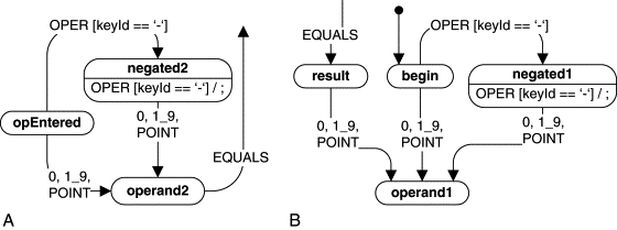
The second case in which − represents the negation is trickier because the specification “beginning of new computation” is much more subtle. Here it indicates the situation just after launching the application or after the user clicks Cancel but not when the calculator displays the result from the previous computation. Figure 2.17(B) shows the solution. A new state “begin” is created to capture the behavior specific to the “beginning of new computation” (note the initial transition pointing now to “begin” rather than to “operand1”). The rest of the solution is analogous as in the first case, except now the state “begin” plays the role of “opEntered.”

The calculator is almost ready now. The final touches (which I leave as an exercise) include adding Cancel-Entry transitions in appropriate contexts and adding an “error” state to capture overflows and division by zero. Figure 2.18 shows the final calculator state diagram. The actual C implementation of this state machine will be described in Chapter 4.

Figure 2.18. The final calculator statechart.