Section 13.1. The Remarkable Utility of (Pseudo)Random Numbers

As discussed in Section 11.1, much of the difficulty that of Big Data analysis comes down to combinatorics. As the number of data objects increases, along with the number of attributes that describe each object, it becomes computationally difficult, or impossible, to compute all the pairwise comparisons that would be necessary for analytics tasks (e.g., clustering algorithms, predictive algorithms). Consequently, Big Data analysts are always on the lookout for innovative, non-combinatoric approaches to traditionally combinatoric problems.

There are many different approaches to data analysis that help us to reduce the complexity of data (e.g., principal component analysis) or transform data into a domain that facilitates various types of analytic procedures (e.g., the Fourier transform). In this chapter, we will be discussing an approach that is easy to learn, easy to implement, and which is particularly well-suited to enormous data sets. The techniques that we will be describing fall under different names, depending on how they are applied (e.g., resampling, Monte Carlo simulations, bootstrapping), but they all make use of random number generators, and they all involve repeated sampling from a large population of data, or from infinite points in a distribution. Together, these heuristic techniques permit us to perform nearly any type of Big Data analysis we might imagine in a few lines of Python code [1–4]. [Glossary Heuristic technique, Principal component analysis]

In this chapter, we will explore:

• –  Random numbers (strictly, pseudorandom numbers) [Glossary Pseudorandom number generator]
• –  General problems of probability
• –  Statistical tests
• –  Monte Carlo simulations
• –  Bayesian models
• –  Methods for determining whether there are multiple populations represented in a data set
• –  Determining the minimal sample size required to test a hypothesis [Glossary Power]
• –  Integration (calculus)

Let us look at how a random number generator works in Python, with a 3-line random.py script.

import random
for iterations in range(10):
 print(random.uniform(0,1))

Here is the sample output, listing 10 random numbers in the range 0–1:

0.594530508550135
0.289645594799927
0.393738321195123
0.648691742041396
0.215592023796071
0.663453594144743
0.427212189295081
0.730280586218356
0.768547788018729
0.906096189758145

Had we chosen, we could have rendered an integer output by multiplying each random number by 10 and rounding up or down to the closest integer.

Now, let us perform a few very simple simulations that confirm what we already know, intuitively. Imagine that you have a pair of dice and you would like to know how often you might expect each of the numbers (from one to six) to appear after you've thrown one die [5].

Let us simulate 60,000 throws of a die using the Python script, randtest.py:

import random, itertools
one_of_six = 0
for i in itertools.repeat(None, 60000):
 if (int(random.uniform(1,7))) > 5:
  one_of_six = one_of_six + 1
print(str(one_of_six))

The script, randtest.pl, begins by setting a loop that repeats 60,000 times, each repeat simulating the cast of a die. With each cast of the die, Python generates a random integer, 1 through 6, simulating the outcome of a throw.

The script yields the total number die casts that would be expected to come up “6.” Here is the output of seven consecutive runs of the randtest.py script

10020
10072
10048
10158
10000
9873
9899

As one might expect, a “6” came up about 1/6th of the time, or about 10,000 times in the 60,000 simulated roles. We could have chosen any of the other five outcomes of a die role (i.e., 1, 2, 3, 4, or 5), and the outcomes would have been about the same.

Let us use a random number generator to calculate the value of pi, without measuring anything, and without resorting to summing an infinite series of numbers. Here is a simple python script, pi.py, that does the job.

import random, itertools
from math import sqrt
totr = 0; totsq = 0
for i in range(10000000):
 x = random.uniform(0,1)
 y = random.uniform(0,1)
 r = sqrt((x⁎x) + (y⁎y))
 if r < 1:
   totr = totr + 1
 totsq = totsq + 1
print(float(totr)⁎4.0/float(totsq))

The script returns a fairly close estimate of pi.

output: 3.1414256

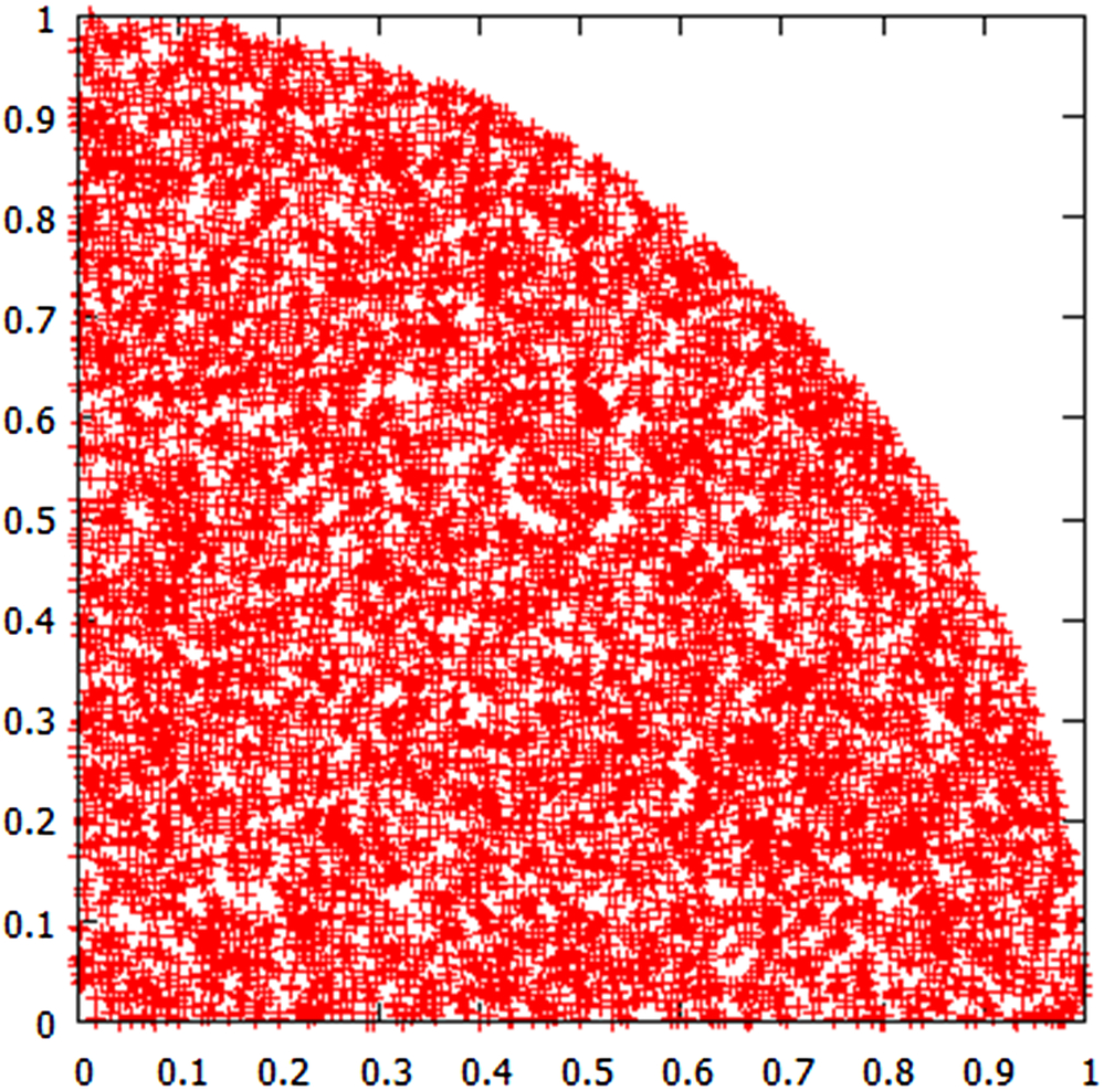
The value of pi is the ratio of a circle of unit radius (pi ⁎ r^∧2) divided by the area of a square of unit radius (rˆ2). When we randomly select points within a unit distance in the x or the y dimension, we are filling up a unit square. When we count the number of randomly selected points within a unit radius of the origin, and compare this number with the number of points in the unit square, we are actually calculating a number that comes fairly close to pi. In this simulation, we are looking at one quadrant, but the results are equivalent, and we come up with a number that is a good approximation of pi (i.e., 3.1414256, in this simulation).

With a few extra lines of code, we can send the output to a to a data file, named pi.dat, that will helps us visualize how the script works. The data output (held in the pi.dat file) contains the x, y data points, generated by the random number generator, meeting the “if” statement's condition that the hypotenuse of the x, y coordinates must be less than one (i.e., less than a circle of radius 1). We can plot the output of the script with a few lines of Gnuplot code:

gnuplot > set size square
gnuplot > unset key
gnuplot > plot 'c:ftppi.dat'

The resulting graph is a quarter-circle within a square (Fig. 13.1).

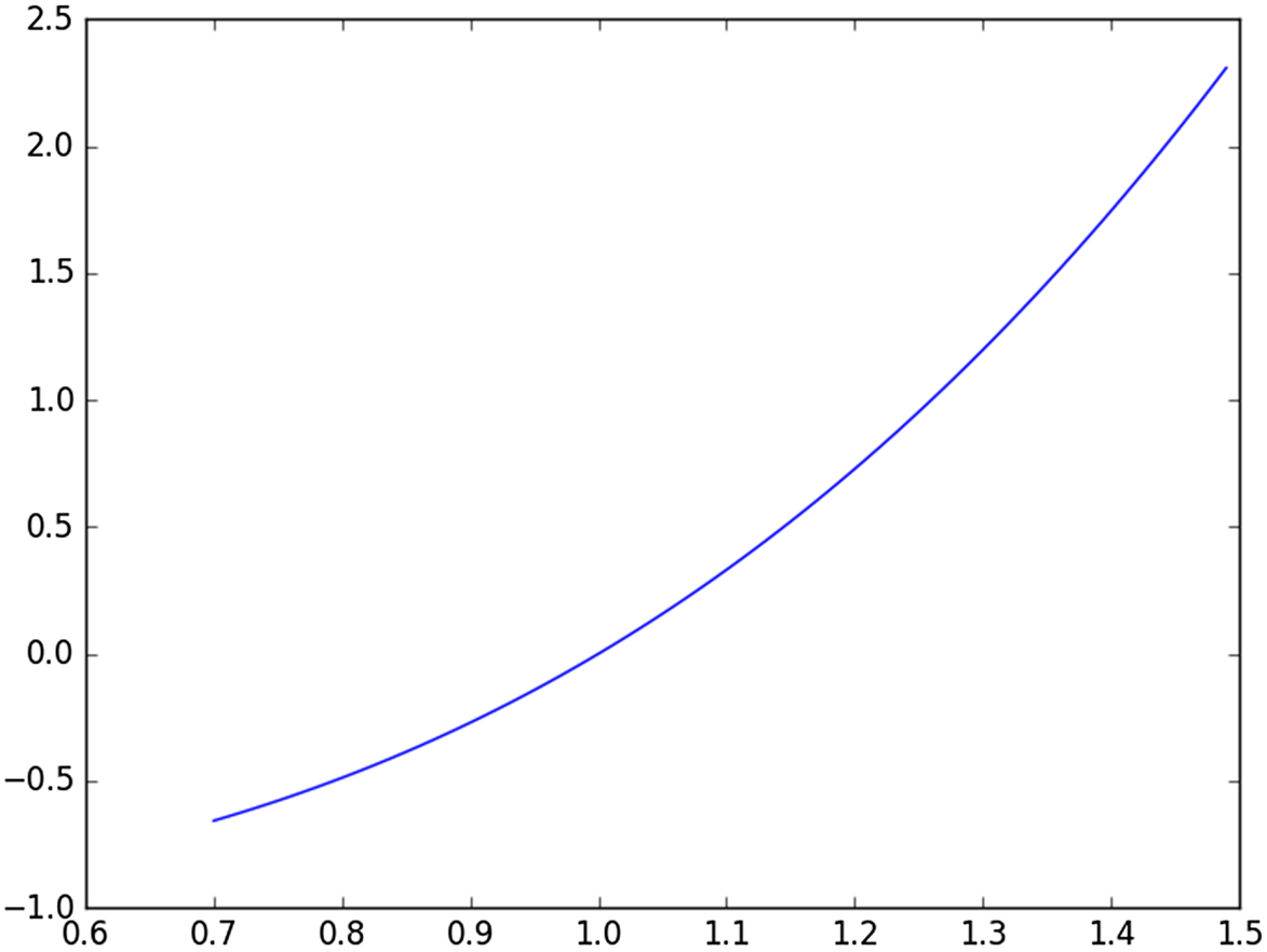
Let us see how we can simulate calculus operations, using a random number generator. We will integrate the expression f(x) = x^∧3 − 1. First, let us visualize the relationship between f(x) and x, by plotting the expression. We can use a very simple Python script, plot_funct.py, that can be trivially generalized to plot almost any expression we choose, over any interval.

import math, random, itertools
import numpy as np
import matplotlib.pyplot as plt
x = 0.000
def f(x):
 return (x⁎x⁎x -1)
x = np.arange(0.7, 1.5, 0.01)
plt.plot(x, f(x))
plt.show()

The output is a graph, produced by Python's matplotlib module (Fig. 13.2).

Let us use a random number generator, in the Python script integrator.py, to perform the integration and produce an approximate evaluation of the integral (i.e., the area under the curve of the equation).

import math, random, itertools
def f(x):
 return (x⁎x⁎x -1)

range = 2   #let's evaluate the integral from x = 1 to x = 3
running_total = 0
for i in itertools.repeat(None, 1000000):
 x = float(random.uniform(1,3))
 running_total = running_total + f(x)
integral = (running_total / 1000000) ⁎ range
print(str(integral))

Here is the output:

18.001426696174935

The output comes very close to the exact integral, 18, calculated for the interval between 1 and 3. How did our short Python script calculate the integral? The integral of a function is equivalent to the area under of the curve of the function, in the chosen interval. The area under the cover is equal to the size of the interval (i.e., the x coordinate range) multiplied by the average value of the function in the interval. By calculating a million values of the function, from randomly chosen values of x in the selected interval, and taking the average of all of those values, we get the average value of the function. When we multiply this by the interval, we get the area, which is equal to the value of the integral.

Let us apply our newfound ability to perform calculus with a random number generator and calculate one of the most famous integrals in mathematics.

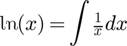
The integral of 1/x equals the natural logarithm of x (Fig. 13.3). This tells us that the integral of (1/x)dx evaluated in the integral from 5 to 105 will be equal to ln(105) minus ln(5). Let us evaluate the integral in the range from x = 5 to x = 105, using our random number generator, alongside the calculation performed with Python's numpy (math) module, to see how close our approximation came. We will use the Python script, natural.py

import math, random, itertools
import numpy as np
def f(x):
 return (1 / x)
range = 100
running_total = 0
for i in itertools.repeat(None, 1000000):
 x = float(random.uniform(5,105))
 running_total = float(running_total + f(x))

integral = (running_total / 1000000) ⁎ range
print("The estimate produced with a random number generator is: " + str(integral))
print("The value produced with Python's numpy function for ln(x) is: " + str(np.log(105) - np.log(5)))

Here is the output of the natural.py script.

The estimate produced with a random number generator is:  3.04209561069317
The value produced with Python's numpy function for ln(x) is: 3.04452243772

Not bad. Of course, python programmers know that they do not need to use a random number generator to solve calculus problems in python. The numpy and sympy modules seem to do the job nicely. Here is a short example wherein the a classic integral equation is demonstrated:

>>> import sympy as sy
>>> import numpy as np
>>> x = sy.Symbol('x')
>>> sy.integrate(1/x,x)
log(x)

Or, as any introductory calculus book would demonstrate: ln x = integral 1/x dx

Why would anyone bother to integrate using a random number generator when they can produce an exact solution using elementary calculus? It happens that integration by repeated sampling using a random number generator comes in handy when dealing with multi-dimensional functions, particularly when the number of dimensions exceeds 8 (i.e., when there are 8 or more quantitative attributes describing each variable). In Big Data, where the variables have many attributes, standard computational approaches may fail. In these cases the methods described in this section may provide the most exact and the most practical solutions to a large set of Big Data computations. [Glossary Curse of dimensionality]

Section 13.2. Repeated Sampling

In Big Data analytics, we can use a random number generator to solve problems in the areas of clustering, correlations, sample size determination, differential equations, integral equations, digital signals processing, and virtually every subdiscipline of physics [3,1,6,5]. Purists would suggest that we should be using formal, exact, and robust mathematical techniques for all these calculations. Maybe so, but there is one general set of problems for which the random number generator is the ideal tool; requiring no special assumptions about the data being explored, and producing answers that are as reliable as anything that can be produced with computationally intensive exact techniques. This set of problems typically consists of hypothesis testing on sets of data of uncertain distribution (i.e., not Gaussian) that are not strictly amenable to classic statistical analysis. The methods by which these problems are solved are the closely related techniques of resampling (from a population or data set) and permutating, both of which employ random number generators. [Glossary Resampling statistics, Permutation test, Resampling versus Repeated Sampling, Modified random sampling]

Resampling methods are not new. The resampling methods that are commonly used today by data analysts have been around since the early 1980s [3,1,2]. The underlying algorithms for these methods are so very simple that they have certainly been in use, using simple casts of dice, for thousands of years.

The early twentieth century saw the rise of mathematically rigorous statistical methods, that enabled scientists to test hypotheses and draw conclusions from small or large collections of data. These tests, which required nothing more than pencil and paper to perform, dominated the field of analysis and are not likely to be replaced anytime soon. Nonetheless, the advent of fast computers provides us with alternative methods of analysis that may lack the rigor of advanced statistics, but have the advantage of being easily comprehensible. Calculations that require millions of operations can be done essentially instantly, and can be programmed with ease. Never before, in the history of the world, has it been possible to design and perform resampling exercises, requiring millions or billions of iterative operations, in a matter of seconds, on computers that are affordable to a vast number of individuals in developed or developing countries. The current literature abounds with resources for scientists with rudimentary programming skills, who might wish to employ resampling techniques [7,8].

For starters, we need to learn a new technique: shuffling. Python's numpy module provides a simple method for shuffling the contents of a container (such as the data objects listed in an array) to produce a random set of objects. Here is Python's shuffle_100.py script, that produces a shuffled list of numbers ranging from 0 to 99:

import numpy as np
sample = np.arange(100)
gather = []
for i in sample:
 np.random.shuffle(sample)
print(sample)

Here is the output of the shuffle_100.py script:

[27 60 21 99 17 79 49 62 81 2 88 90 45 61 66 80 50 31 59 24 53 29 64 33 30
 41 13 23 0 67 78 70 1 35 18 86 25 93 6 98 97 84 9 12 56 48 74 96 4 32

 44 11 19 38 26 52 87 77 39 91 92 76 65 75 63 57 8 94 51 69 71 7 73 34 20
 40 68 22 82 15 37 72 28 47 95 54 55 58 5 3 89 46 85 16 42 36 43 10 83 14]

We will be using the shuffle method to help us answer a question that arises often, whenever we examine sets of data: “Does my data represent samples from one homogeneous population of data objects, or does my data represent samples from different classes of data objects that have been blended together in one collection?” The blending of distinctive classes of data into one data set is one of the most formidable biases in experimental design, and has resulted in the failures of many clinical trials, the misclassification of diseases, and the misinterpretation of the significance of outliers. How often do we fail to understand our data, simply because we cannot see the different populations lurking within? In Section 12.6, we discussed the importance of finding multimodal peaks in data distributions. Our discussion of multimodal peaks and separable subpopulations begged the question as to how we can distinguish peaks that represent subpopulations from peaks that represent random perturbations in our data. [Glossary Blended class]

Let us begin by using a random number generator to make two separate populations of data objects. The first population of data objects will have values that range uniformly between 1 and 80. The second population of data objects will have values that range uniformly between 20 and 100. These two populations will overlap (between 20 and 80), but they are different populations, with different population means, and different sets of properties that must account for their differences in values. We'll call the population ranging from 1 to 80 our low_array and the population ranging from 20 to 100 as high_array.

Here is a Python script, low_high.py, that generates the two sets of data, representing 50 randomly selected objects from each population:

import numpy as np
from random import randint
low_array = []; high_array = []
for i in range(50):
 low_array.append(randint(1,80))
print("Here's the low-skewed data set " + str(low_array))
for i in range(50):
 high_array.append(randint(21,100))
print("
Here's the high-skewed data set " + str(high_array))
av_diff = (sum(high_array)/len(high_array)) - (sum(low_array)/len(low_array))
print("
The difference in average value of the two arrays is:" + str(av_diff))

Here is the output of the low_high.py script:

Here is the low-skewed data set [31, 8, 60, 4, 64, 35, 49, 80, 6, 9, 14, 15, 50, 45, 61, 77, 58, 24, 54, 45, 44, 6, 78, 59, 44, 61, 56, 8, 30, 34, 72, 33, 14, 13, 45, 10, 49, 65, 4, 51, 25, 6, 37, 63, 19, 74, 78, 55, 34, 22]

Here is the high-skewed data set [36, 87, 54, 98, 33, 49, 37, 35, 100, 48, 71, 86, 76, 93, 98, 99, 92, 68, 29, 34, 64, 30, 99, 76, 71, 32, 77, 32, 73, 54, 34, 44, 37, 98, 42, 81, 84, 56, 55, 85, 55, 22, 98, 72, 89, 24, 43, 76, 87, 61]
The difference in average value of the two arrays is: 23.919999999999995

The low-skewed data set consists of 50 random integers selected from the interval 1–80. The high-skewed data set consists of 50 random numbers selected from the interval between 20 and 100. Notice that not all possible outcomes in these two intervals are represented (i.e., there is no number 2 in the low-skewed data set and there is no number 25 in the high-skewed data set). If we were to repeat the low_high.py script, we would generate two different sets of numbers. Also, notice that the two populations have different average values. The difference between the average value of the low-skewed data population and the high-skewed data population is 23.9, in this particular simulation.

Now, we are just about ready to determine whether the two populations are statistically different. Let us repeat the simulation. This time, we will combine the two sets of data into one array that we will call “total_array,” containing 100 data elements. Then we will shuffle all of the values in total_array and we will create two new arrays: a left array consisting of the first 50 values in the shuffled total_array and a right array consisting of the last 50 values in the total_array. Then we will find the difference between the average of the 50 values of the left array of the right array. We will repeat this 100 times, printing out the lowest five differences in averages and the highest five differences in averages. Then we will stop and contemplate what we have done.

Here is the Python script, pop_diff.py

import numpy as np
from random import randint
low_array = []
high_array = []
gather = []
for i in range(50):
 low_array.append(randint(1,80))
for i in range(50):
 high_array.append(randint(21,100))
av_diff = (sum(high_array)/len(high_array)) - (sum(low_array)/len(low_array))
print("The difference in the average value of the high and low arrays is: " + str(av_diff))
sample = low_array + high_array
for i in sample:
 np.random.shuffle(sample)
 right = sample[50:]

 left = sample[:50]
 gather.append(abs((sum(left)/len(left)) - (sum(right)/len(right))))
sorted_gather = sorted(gather)
print("The 5 largest differences of averages of the shuffled arrays are:")
print(str(sorted_gather[95:]))
output:
The difference in the average value of the high and low arrays is: 19.580000000000005
The 5 largest differences of averages of the shuffled arrays are:
 [8.780000000000001, 8.899999999999999, 9.46, 9.82, 9.899999999999999]

Believe it or not, we just demonstrated that the two arrays that we began with (i.e., the array with data values randomly distributed between 0 and 80; and the array with data values randomly distributed between 20 and 100) represent two different populations of data (i.e., two separable classes of data objects). Here is what we did and how we reached our conclusion.

1. 1.  We recomputed two new arrays, with 50 items each, with data values randomly distributed between 0 and 80; and the array with data values randomly distributed between 20 and 100.
2. 2.  We calculated the difference of the average size of an item in the first array, compared with the average size of an item in the second array. This came out to 19.58 in this simulation.
3. 3.  We combined the two arrays into a new array of 100 items, and we shuffled these items 100 times, each time splitting the shuffle in half to produce two new arrays of 50 items each., We calculated the difference in the average value of the two arrays (produced by the shuffle).
4. 4.  We found the five sets of shuffled arrays (the two arrays produced by a shuffle of the combined array) that had the largest differences in their values (corresponding to the upper 5% of the combined and shuffled populations) and we printed these numbers.

The upper 5 percentile differences among the shuffled arrays (i.e., 8.78, 8.89, 9.46, 9.82, 9.89) came nowhere close to the difference of 19.58 we calculated for the original two sets of data. This tells us that whenever we shuffle the combined array, we never encounter differences anywhere near as great as what we observed in the original arrays. Hence, the original two arrays cannot be explained by random selection from one population (obtained when we combined the two original arrays). The two original arrays must represent two different populations of data objects.

A note of caution regarding scalability. Shuffling is not a particularly scalable function [9]. Shuffling a hundred items is a lot easier than shuffling a million items. Hence, when writing short programs that test whether two data arrays are statistically separable, it is best to impose a limit to the size of the arrays that you create when you sample from the combined array. If you keep the shuffling size small, you can compensate by repeating the shuffle nearly as often as you like.

• –  Sample Size and Power Estimates

In the prior exercise, we generated two populations, of 50 samples each, and we determined that the two populations were statistically separable from one another. Would we have been able to draw the same conclusion if we had performed the exercise using 25 samples in each population in each population? How about 10 samples? We would expect that as the population sizes of the two populations shrinks, the likelihood that we could reliably distinguish one population from another will fall. How do we determine the minimal population size necessary to perform our experiment?

The power of a trial is the likelihood of detecting a difference in two populations, if the difference actually exists. The power is related to the sample size. At a sufficiently large sample size, you can be virtually certain that the difference will be found, if the difference exists. Resampling permits the experimenter to conduct repeated trials, with different sample sizes, and under conditions that simulate the population differences that are expected. For example, an experimenter might expect that a certain drug produces a 15% difference in the measured outcomes in the treated population compared with the control population. By setting the conditions of the trials, and by performing repeated trials with increasing sizes of simulated populations, the data scientist can determine the minimum sampling size that consistently (e.g., in greater than 95% of the trials), demonstrates that the treated population and the control population are separable. Hence, using a random number generator and a few short scripts, the data scientist can determine the sampling size required to yield a power that is acceptable for a “real” experiment. [Glossary Sample size, Sampling theorem]

Section 13.3. Monte Carlo Simulations

Random number generators are well suited to Monte Carlo simulations, a technique described in 1946 by John von Neumann, Stan Ulam, and Nick Metropolis [10]. For these simulations, the computer generates random numbers and uses the resultant values to represent outcomes for repeated trials of a probabilistic event. Monte Carlo simulations can easily simulate various processes (e.g., Markov models and Poisson processes) and can be used to solve a wide range of problems [11,12].

For example, consider how biologists may want to model the growth of clonal colonies of cells. In the simplest case, wherein cell growth is continuous, a single cell divides, producing two cells. Each of the daughter cells divides, producing a total of four cells. The size of the colony increases as powers of 2. A single liver cancer cell happens to have a volume of about 30,000 cubic microns [13]. If the cell cycle time is one day, then the volume of a liver cell colony, grown for 45 days, and starting at day 1 with a single cell, would be 1 m³. In 55 days, the volume would exceed 1000 m³. If an unregulated tumor composed of malignant liver cells were to grow for the normal lifetime of a human, it would come to occupy much of the measured universe [14]. Obviously, unregulated cellular growth is unsustainable. In tumors, as in all systems that model the growth of cells and cellular organisms, the rate of cell growth is countered by the rate of cell death.

With the help of a random number generator, we can model the growth of colonies of cells by assigning each cell in the colony a probability of dying. If we say that the likelihood that a cell will die is 50%, then we are saying that its chance of dividing (i.e., producing two cells) is the same as its chance of dying (i.e., producing zero cells and thus eliminating itself from the population). We can create a Monte Carlo simulation of cell growth by starting with some arbitrary number of cells (let us say three), and assigning each cell an arbitrary chance of dying (let us say 49%). We can assign each imaginary cell to an array, and we can iterate through the array, cell by cell. As we iterate over each cell, we can use a random number generator to produce a number between 0 and 1. If the random number is less than 0.49, we say that the cell must die, dropping out of the array. If a cell is randomly assigned a number that is greater than 0.49, then we say that the cell can reproduce, to produce two cells that will take their place in the array. Every iteration over the cells in the array produces a new array, composed of the lucky winners and their offspring, from the prior array. In theory, we can repeat this process forever. More practically, we can repeat this process until the size of the colony reduces to zero, or until the colony becomes so large that additional iterations become tedious (even for a computer).

Here is the Python script, clone.py, that creates a Monte Carlo simulation for the growth of a colony, beginning with three cells, with a likelihood of cell death for all cells, during any generation, of 0.41. The script exits if the clone size dwindles to zero (i.e., dies out) or reaches a size exceeding 800 (presumably on the way to growing without limit).

import numpy.random as npr
import sys
death_chance = 0.41; cell_array = [1, 1, 1]; cell_array_incremented = [1,1,1]
while(len(cell_array) > 0):
 for cell in cell_array:
    randnum = npr.randint(1,101)
    if randnum > 100 ⁎ death_chance:
     cell_array_incremented.append(1)
    else:
     cell_array_incremented.remove(1)
 if len(cell_array_incremented) < 1:
   sys.exit()

 if len(cell_array_incremented) > 800:
   sys.exit()
 cell_array = cell_array_incremented
 print(len(cell_array_incremented), end = ", ")

For each cell in the array, if the random number generated for the cell exceeds the likelihood of cell death, then the colony array is incremented by one. Otherwise, the colony array is decremented by 1. This simple step is repeated for every cell in the colony array, and is repeated for every clonal generation.

Here is a sample output when death_chance = 0.49

multiple outputs:
First trial:
2, 1, 1, 1,
Second trial:
4, 3, 3, 1,
Third trial:
6, 12, 8, 15, 16, 21, 30, 37, 47, 61, 64, 71, 91, 111, 141, 178, 216, 254, 310, 417, 497, 597, 712,
Fourth trial:
2, 4, 4, 4, 3, 3, 4, 4, 8, 5, 6, 4, 4, 6, 4, 10, 19, 17, 15, 32, 37, 53, 83, 96, 128, 167, 188, 224, 273, 324, 368, 416, 520, 642,
Fifth trial
4, 3, 7, 9, 19, 19, 26, 36, 45, 71, 88, 111, 119, 157, 214, 254, 319, 390, 480, 568, 675,
Sixth trial:
2, 1, 2, 2, 1,
Seventh trial:
2, 1,
Eighth trial:
2, 1, 1, 1, 4, 8, 10, 8, 10, 9, 10, 15, 11, 12, 16, 15, 21, 21, 35, 44, 43, 41, 47, 68, 62, 69, 90, 97, 121, 181, 229, 271, 336, 439, 501, 617, 786,

In each case the clone increases or decreases with each cell cycle until the clone reaches extinction or exceeds our cut off limit. These simulations indicate that clonal growth is precarious, under conditions when the cell death probability is approximately 50%. In these two simulations the early clones eventually die out. Had we repeated the simulation hundreds of times, we would have seen that most clonal simulations end in the extinction of the clone; while a few rare simulations yield a large, continuously expanding population, with virtually no chance of reaching extinction. In a series of papers by Dr. William Moore and myself, we developed Monte Carlo simulations of tumor cell growth. Those simulations suggested that very small changes in a tumor cell's death probability (per replication generation) profoundly affected the tumor's growth rate [11,12,15]. This simulation suggested that chemotherapeutic agents that can incrementally increase the death rate of tumor cells may have enormous treatment benefit. Furthermore, simulations showed that if you simulate the growth of a cancer from a single abnormal cancer cell, most simulations result in the spontaneous extinction of the tumor, an unexpected finding that helps us to understand the observed high spontaneous regression rate of nascent growths that precede the development of clinically malignant cancers [16,17].

This example demonstrates how simple Monte Carlo simulations, written in little more than a dozen lines of Python code, can simulate outcomes that would be difficult to compute using any other means.

Section 13.4. Case Study: Proving the Central Limit Theorem

The Central Limit Theorem is a key concept in probability theory and statistics. It asserts that when independent random variables are added, their sum tends toward a normal distribution (i.e., a “bell curve”). The importance of this theorem is that statistical methods designed for normal distributions will also apply in some situations wherein variables are chosen randomly from non-normal distributions.

For many years, the Central Limit Theorem was a personal stumbling block for me; I simply could not understand why it was true. It seemed to me that if you randomly select numbers in an interval, you would always get a random number, and if you summed and averaged two random numbers, you'll get another random number that is equally likely to by anywhere within the interval (i.e., not distributed along a bell curve with a central peak). According to the Central Limit Theorem, the sum of repeated random samplings will produce lots of numbers in the center of the interval, and very few or no numbers at the extremes.

As previously mentioned, repeated sampling allows us to draw inferences about a population, without examining every member of the population; a handy trick for Big Data analyses. In addition, repeated sampling allows us to test hypotheses that we are too dumb to understand (speaking for myself). In the case of the Central Limit Theorem, we can simulate a proof of the Central Limit Theorem by randomly selecting numbers in an interval (between 0 and 1) many times (say 10,000), and averaging their sum. We can repeat each of these trials 10,000 times, and then plot where the 10,000 values lie. If we get a Bell curve, then the Central Limit Theorem must be correct. Here is the Python script, central.py, that computes the results of the simulation, and plots the points as a graph.

import random, itertools
from matplotlib import numpy
import matplotlib.pyplot as plt
out_file = open('central.dat',"w")
randhash = {}
for i in itertools.repeat(None, 10000):
 product = 0
 for n in itertools.repeat(None, 10000):
   product = product + random.uniform(0,1)
 product = int(product)
 if product in randhash:
   randhash[product] = randhash[product] + 1
 else:
   randhash[product] = 1
lists = sorted(randhash.items())
x, y = zip(⁎lists)
plt.plot(x, y)
plt.show()

Here is the resultant graph (Fig. 13.4).

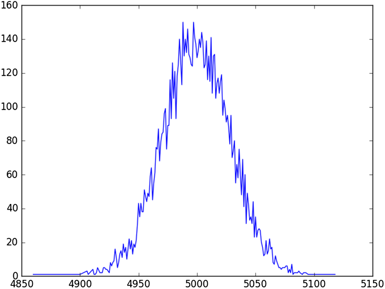
Without bludgeoning the point, after performing the simulation, and looking at the results, the Central Limit Theorem suddenly makes perfect sense to me. The reader can draw her own conclusion.

Section 13.5. Case Study: Frequency of Unlikely String of Occurrences

Imagine this scenario. A waitress drops a serving tray three times while serving each of three consecutive customers on the same day. Her boss tells her that she is incompetent, and indicates that he should fire her on the spot. The waitress objects, saying that the other staff drops trays all the time. Why should she be singled out for punishment simply because she had the bad luck of dropping three trays in a row. The manager and the waitress review the restaurant's records and find that there is a 2% drop rate, overall (i.e., a tray is dropped 2% of the time when serving customers), and that the waitress who dropped the three trays in one afternoon had had a low drop rate prior to this day's performance. She cannot explain why three trays dropped consecutively, but she supposes that if anyone works the job long enough, the day will come when they drop three consecutive trays.

We can resolve this issue, very easily, with the Python script runs.py, that simulates a million customer wait services and determines how often we are likely to see a string of three consecutive dropped trays.

import random, itertools
errorno = 0;
for i in itertools.repeat(None, 1000000): #let's do 1 million table services
 x = int(random.uniform(0,100))   #x any integer from 0 to 99
 if (x < 2):       #x simulates a 2% error rate
   errorno = errorno + 1
 else:
   errorno = 0
 if (errorno == 3):
   print("Uh oh. 3 consecutive errors")
   errorno = 0

Here is the output from one execution of runs.py

Uh oh. 3 consecutive errors
Uh oh. 3 consecutive errors
Uh oh. 3 consecutive errors
Uh oh. 3 consecutive errors

Uh oh. 3 consecutive errors
Uh oh. 3 consecutive errors
Uh oh. 3 consecutive errors
Uh oh. 3 consecutive errors

The 11-line Python script simulates 1 million table services. Each service is assigned a random number between 0 and 100. If the randomly assigned number is less than 2 the simulation counts as a dropped tray (because the drop rate is 2%). Now we watch to see the outcome of the next two served trays. If three consecutive trays are dropped, we print out “Uh oh. 3 consecutive errors”) and we resume our simulations.

In this trial of 1 million table services, using a 2% error rate, the modeled waitress had eight runs of three consecutive tray drops. Since a million table services might possibly represent the total number of customers served by a waitress in her entire career, one can say that she should be allowed at least eight episodes of three consecutive tray drops, in her lifetime.

Section 13.6. Case Study: The Infamous Birthday Problem

Let us use our random number generator to tackle the infamous birthday problem. It may seem unintuitive, but if you have a room holding 23 people, the odds are about even that two or more of the group will share the same birth date. The solution of the birthday problem has become a popular lesson in introductory probability courses. The answer involves an onerous calculation, involving lots of multiplied values, divided by an enormous exponential (Fig. 13.5).

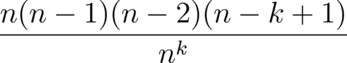
If we wanted to know the probability of finding two or more individuals with the same birthday, in a group of 30 individuals, we could substitute 365 for n and 30 for k, and we would learn that the odds are about 70%. Or, we could design a simple little program, using a random number generator, to create an intuitively obvious simulation of the problem.

Here is the Python script, birthday.py, that conducts 10,000 random simulations of the birthday problem:

import random, itertools
success = 0
for i in itertools.repeat(None, 10000):

 date_hash = {}
 for j in itertools.repeat(None, 30):
  date = int(random.uniform(1,365))
  if date in date_hash:
   date_hash[date] = date_hash[date] + 1
  else:
   date_hash[date] = 1
  if (date_hash[date] == 2):
   success = success + 1
   break
print(str(success / 10000))

Here is the output from six consecutive runs of birthday.py, with 10,000 trials in each run:

0.7076
0.7083
0.7067
0.7101
0.7087
0.7102

The calculated probability is about 70%. The birthday.py script created variables, assigning each variable a birth date selected at random from a range of 1–365 (the number of days in the year). The script then checked among the 30 assigned variables, to see if any of them shared the same birthday (i.e., the same randomly assigned number). If so, then the set of 30 assigned variables was deemed a success. The script repeated this exercise 10,000 times, incrementing, by one, the number of successes whenever a match was found in the 30 assignments. At the end of it all, the total number of successes (i.e., instances where there is a birthday match in the group of 30) divided by the total number of simulations (10,000 in this case) provides the likelihood that any given simulation will find a birthday match. The answer, which happens to be about 70%, is achieved without the use of any knowledge of probability theory.

Section 13.7. Case Study (Advanced): The Monty Hall Problem

This is the legendary Monty Hall problem, named after the host of a televised quiz show, where contestants faced a similar problem: “The player faces three closed containers, one containing a prize and two empty. After the player chooses, s/he is shown that one of the other two containers is empty. The player is now given the option of switching from her/his original choice to the other closed container. Should s/he do so? Answer: Switching will double the chances of winning.”

Marilyn vos Savant, touted by some as the world's smartest person, correctly solved the Monty Hall problem in her newspaper column. When she published her solution, she received thousands of responses, many from mathematicians, disputing her answer.

Basically, this is one of those rare problems that seems to defy common sense. Personally, whenever I have approached this problem using an analytic approach based on probability theory, I come up with the wrong answer.

In desperation, I decided to forget everything I thought I knew about probability, in favor of performing the Monty Hall game, with a 10-line Python script, montyhall.py, that uses a random number generator to simulate outcomes.

import random, itertools
winner = 0; box_array = [1,2,3]
for i in itertools.repeat(None, 10000):
 full_box = int(random.uniform(1,4))  #randomly picks 1,2,or 3 as prize box
  guess_box = int(random.uniform(1,4))#represents your guess, for prize box
 del box_array[full_box - 1]      #prize box deletes itself from array
 if guess_box in box_array:      #if your first guess is in the remaining array
                      #(which excludes prize and includes the second
                      #empty box), then you must have won
                      #when you chose to switch your choice
  winner = winner + 1
 box_array = [1,2,3]
print(winner)

Here are the outputs of nine consecutive runs of montyhall.py script:

6710
6596
6657
6698
6653
6684
6661
6607
6674

The script simulates the Monty Hall strategy where the player takes the option of switching her selection. By taking the switch option, she wins nearly two thirds of the time (about 6600 wins in 10,000 simulations), twice as often as when the switch option is declined. The beauty of the resampling approach is that the programmer does not need to understand why it works. The programmer only needs to know how to use a random number generator to create an accurate simulation of the Monte Hall problem that can be repeated thousands and thousands of times.

How does the Monty Hall problem relate to Big Data? Preliminary outcomes of experimental trials are often so dramatic that the trialists choose to re-design their protocol mid-trial. For example, a drug or drug combination may have demonstrated sufficient effectiveness to justify moving control patients into the treated group. Or adverse reactions may necessitate switching patients off a certain trial arm. In either case, the decision to switch protocols based on mid-trial observations is a Monty Hall scenario.

Section 13.8. Case Study (Advanced): A Bayesian Analysis

The Bayes theorem relates probabilities of events that are conditional upon one another (Fig. 13.6). Specifically, the probability of A occurring given that B has occurred multiplied by the probability that B occurs is equal to the probability of B occurring, given that A has occurred multiplied by the probability that A occurs. Despite all the hype surrounding Bayes theorem, it basically indicates the obvious: that if A and B are conditional, then A won't occur unless B occurs and B won't occur unless A occurs.

Bayesian inferences involve computing conditional probabilities, based on having information about the likelihood of underlying events. For example, the probability of rain would be increased if it were known that the sky is cloudy. The fundamentals of Bayesian analysis are deceptively simple. In practice, Bayesian analysis can easily evade the grasp of intelligent data scientists. By simulating repeated trials, using a random number generator, some of the toughest Bayesian inferences can be computed in a manner that is easily understood, without resorting to any statistical methods.

Here is a problem that was previously posed by William Feller, and adapted for resampling statistics by Julian L. Simon [1]. Imagine a world wherein there are two classes of drivers. One class, the good drivers, comprise 80% of the population, and the likelihood that a member of this class will crash his car is 0.06 per year. The other class, the bad drivers, comprise 20% of the population, and the likelihood that a member of this class will crash his car is 0.6 per year. An insurance company charges clients $100 times the likelihood of having an accident, as expressed as a percentage. Hence, a member of the good driver class would pay $600 per year; a member of the bad driver class would pay $6000 per year. The question is: If nothing is known about a driver other than that he had an accident in the prior year, then what should he be charged for his annual car insurance payment?

The Python script, bayes.py, calculates the insurance cost, based on 10,000 trial simulations:

import random, itertools
accidents_next_year = 0
no_accidents_next_year = 0
for i in itertools.repeat(None, 10000):
 group_likelihood = random.uniform(0,1)
 if (group_likelihood < 0.2):       #puts trial in poor-judgment group
   bad_likelihood = random.uniform(0,1) #roll the dice to see if accident occurs
   if (bad_likelihood < 0.6):       #an accident occurred, simulating an initial
                       #condition of poor-judgment with accident
    next_bad_likelihood = random.uniform(0,1)
    if (next_bad_likelihood < 0.6):
     accidents_next_year = accidents_next_year + 1
    else:
     no_accidents_next_year = no_accidents_next_year + 1
 else: #othwerwise we bump the trial into the good-judgment group
   bad_likelihood = random.uniform(0,1) #simulates an accident accident
   if (bad_likelihood < 0.06):      #an accident with good-judgment
    next_bad_likelihood = random.uniform(0,1)
    if (next_bad_likelihood < 0.06):
     accidents_next_year = accidents_next_year + 1
    else:
     no_accidents_next_year = no_accidents_next_year + 1
cost = int(((accidents_next_year)/(accidents_next_year + no_accidents_next_year)⁎100⁎100))
print("Insurance cost is $" + str(cost))

outputs of 7 executions of bayes.py script:
Insurance cost is 4352
Insurance cost is 4487
Insurance cost is 4406
Insurance cost is 4552
Insurance cost is 4454
Insurance cost is 4583
Insurance cost is 4471

In all eight executions of the script, each having 10,000 trials, we find that the insurance cost, based on initial conditions, should be about $4500.

What does our bayes.py do? First, it creates a loop for 10,000 trial simulations. Within each simulation, it begins by choosing a random number between 0 and 1. If the random number is less than 0.2, then this simulates an encounter with a member of the bad-driver class (i.e., the bottom 20% of the population). In this case the random number generator produces another number between 0 and 1. If this number is less than 0.6 (the annual likelihood of a bad driver having an accident), then this would be simulate a member of the bad-driver class who had an accident and who is applying for car insurance. Now, we run the random number generator one more time, to simulate whether the bad driver will have an accident during the insurance year. If the generated random number is less than 0.6, we will consider this a simulation of a bad-driver, who had an accident prior to asking for applying for car insurance, having an accident in the subsequent year. We will do the same for the simulations that apply to the good drivers (i.e., the trials for which our group likelihood random number was greater than 0.2). After the simulations have looped 10,000 times, all that remains is to use our tallies to calculate the likelihood of an accident, which in turn gives us the insurance cost. In this example, as in all our other examples, we really did not need to know any statistics. We only needed to know the conditions of the problem, and how to simulate those conditions as Monte Carlo trials.

Glossary

Blended class Also known as class noise. Blended class refers to inaccuracies (e.g., misleading results) introduced in the analysis of data due to errors in class assignments (e.g., inaccurate diagnosis). If you are testing the effectiveness of an antibiotic on a class of people with bacterial pneumonia, the accuracy of your results will be forfeit when your study population includes subjects with viral pneumonia, or smoking-related lung damage. Errors induced by blending classes are often overlooked by data analysts who incorrectly assume that the experiment was designed to ensure that each data group is composed of a uniform and representative population. A common source of class blending occurs when the classification upon which the experiment is designed is itself blended. For example, imagine that you are a cancer researcher and you want to perform a study of patients with malignant fibrous histiocytomas (MFH), comparing the clinical course of these patients with the clinical course of patients who have other types of tumors. Let us imagine that the class of tumors known as MFH does not actually exist; that it is a grab-bag term erroneously assigned to a variety of other tumors that happened to look similar to one another. This being the case, it would be impossible to produce any valid results based on a study of patients diagnosed as MFH. The results would be a biased and irreproducible cacophony of data collected across different, and undetermined, classes tumors. Believe it or not, this specific example, of the blended MFH class of tumors, is selected from the real-life annals of tumor biology [18–20]. The literature is rife with research of dubious quality, based on poorly designed classifications and blended classes. One caveat; efforts to reduce class blending can be counterproductive if undertaken with excess zeal. For example, in an effort to reduce class blending, a researcher may choose groups of subjects who are uniform with respect to every known observable property. For example, suppose you want to actually compare apples with oranges. To avoid class blending, you might want to make very sure that your apples do not included any cumquats, or persimmons. You should be certain that your oranges do not include any limes or grapefruits. Imagine that you go even further, choosing only apples and oranges of one variety (e.g., Macintosh apples and Navel oranges), size (e.g., 10 cm), and origin (e.g., California). How will your comparisons apply to the varieties of apples and oranges that you have excluded from your study? You may actually reach conclusions that are invalid and irreproducible for more generalized populations within each class. In this case, you have succeeded in eliminated class blending at the expense of having representative populations of the classes.

Curse of dimensionality As the number of attributes for a data object increases, the distance between data objects grows to enormous size. The multidimensional space becomes sparsely populated, and the distance between any two objects, even the two closest neighbors, becomes absurdly large. When you have thousands of dimensions, the space that holds the objects is so large that distances between objects become difficult or impossible to compute, and computational products become useless for most purposes.

Heuristic technique A way to solve problems with inexact but quick methods, sufficient for most practical purposes.

Modified random sampling When we think of random sampling, we envision a simple, unbiased random selection from all the data objects within a collection. Consider a population of 7 billion people, where the number of individuals aged 60 and above account for 75% of the population. A random sampling of this population would be skewed to select senior citizens, and might yield very few children in kindergarten. Depending on the study, the data analyst may want to change the sampling rules to attain a random sampling that produces a population that fits the study goals. In this example the population might be partitioned into age groups (by decade), with an individual in any partitioned group having the same chance of being randomly selected as an individual in any other partitioned age group.
There are many different ways in which the rules of random sampling can be modified to accommodate an analytic approach [21]. Here are a few:
– Event-based sampling, in which data are collected only at specific moments, when the data being received meet particular criteria or exceed a preset threshold
– Adaptive random sampling, in which the rules for selection are determined by prior observations on the selected samples
– Attribute-based sampling, in which the probability of selection is weighted by a feature attribute of a data object
Of course, when we introduce a modification to the simple process of random selection, we risk introducing new and unexpected biases and confounders, and we open ourselves to criticism and the possibility that our conclusions cannot be repeated in other populations. It is another of those damned if you do and damned if you don't scenarios that we can expect in nearly every Big Data analysis.

Permutation test A method whereby the null hypothesis is accepted or rejected after testing all possible outcomes under rearrangements of the observed data elements.

Power In statistics, power describes the likelihood that a test will detect an effect, if the effect actually exists. In many cases, power reflects sample size. The larger the sample size, the more likely that an experiment will detect a true effect; thus correctly rejecting the null hypothesis.

Principal component analysis One popular methods for transforming data to reduce the dimensionality of data objects is multidimensional scaling, which employs principal component analysis [22]. Without going into the mathematics, principal component analysis takes a list of parameters and reduces it to a smaller list, with each component of the smaller list constructed from variables in the longer list (as a sum of variables multiplied by weighted coefficients). Furthermore, principal component analysis provides an indication of which variables are least correlated with the other variables (as determined by the size of the coefficients). Principal component analysis requires operations on large matrices. Such operations are computationally intensive and can easily exceed the capacity of most computers [22].

Pseudorandom number generator It is impossible for computers to produce an endless collection of truly random numbers. Eventually, algorithms will cycle through their available variations and begins to repeat themselves, producing the same set of “random” numbers, in the same order; a phenomenon referred to as the generator's period. Because algorithms that produce seemingly random numbers are imperfect, they are known as pseudorandom number generators. The Mersenne Twister algorithm, which has an extremely long period, is used as the default random number generator in Python. This algorithm performs well on most of the tests that mathematicians have devised to test randomness.

Resampling statistics A technique whereby a sampling of observations is artifactually expanded by randomly selecting observations and adding them to the original data set; or by creating new sets of data by randomly selecting, without removing, data elements from the original data.

Resampling versus Repeated Sampling In resampling statistics, a limited number of data measurements is expanded by randomly selecting data and adding them back to the original data. In Big Data, there are so many data points that statistical tools cannot quickly evaluate them. Repeated sampling involves randomly selecting subpopulations of enormous data sets, over and over again, and performing statistical evaluations on these multiple samplings, to arrive at some reasonable estimate of the behavior of the entire set of data. Although random sampling is involved in resampling statistics and repeated sampling statistics, the latter does not resample the same data points.

Sample size The number of samples used in a study. Methods are available for calculating the required sample size to rule out the null hypothesis, when an effect is present at a specified significance level, in a population with a known population mean, and a known standard deviation [23]. The sample size formula should not be confused with the sampling theorem, which deals with the rate of sampling that would be required to adequately digitize an analog (e.g., physical or electromagnetic) signal.

Sampling theorem A foundational principle of digital signal processing, also known as the Shannon sampling theorem or the Nyquist sampling theorem. The theorem states that a continuous signal can be properly sampled, only if it does not contain components with frequencies exceeding one-half of the sampling rate. For example, if you want to sample at a rate of 4000 samples per second, you would prefer a signal containing no frequencies greater than 2000 cycles per second.