Section 11.1. Speed and Scalability

Speed and scalability are the two issues that never seem to go away when discussions turn to Big Data. Will we be able to collect, organize, search, retrieve, and analyze Big Data at the same speed that we have grown accustomed to in small data systems? Will the same algorithms, software, protocols, and systems that work well with small data scale up to Big Data?

Let us turn the question around for a moment. Will Big Data solutions scale down to provide reliable and fast solutions for small data? It may seem as though the answer is obvious. If a solution works for large data it must also work for small data. Actually, this is not the case. Methods that employ repeated sampling of a population may produce meaningless results when the population consists of a dozen data points. Nonsensical results can be expected when methods that determine trends, or analyze signals come up against small data.

The point here is that computational success is always an artifact of the way that we approach data-related issues. By customizing solutions to some particular set of circumstances (number of samples, number of attributes, required response time, required precision), we make our products ungeneralizable. We tend to individualize our work, at first, because we fail to see the downside of idiosyncratic solutions. Hence, we learn the hard way that solutions that work well under one set of circumstances will fail miserably when the situation changes. Desperate to adapt to the new circumstances, we often pick solutions that are expensive and somewhat short-sighted (e.g., “Let's chuck all our desktop computers and buy a supercomputer.”; “Let's parallelize our problems and distribute the calculations to multiple computers”, “Let's forget about trying to understand the system and switch to deep learning with neural networks.”; “Let's purchase a new and more powerful information system and abandon our legacy data.”)

In this book, which offers a low-tech approach to Big Data, we have been stressing the advantages of simple and general concepts that allow data to be organized at any level of size and complexity (e.g., identifiers, metadata/data pairs, triples, triplestores), and extremely simple algorithms for searching, retrieving, and analyzing data that can be accomplished with a few lines of code in any programming language. The solutions discussed in this book may not be suitable for everyone, but it is highly likely that many of the difficulties associated with Big Data could be eliminated or ameliorated, if all data were well organized.

Aside from issues of data organization, here are a few specific suggestions for avoiding some of the obstacles that get in the way of computational speed and scalability:

• –  High-level programming languages (including Python) employ built-in methods that fail when the variables are large, and such methods must be avoided by programmers.

Modern programming languages relieve programmers from the tedium of allocating memory to every variable. The language environment is tailored to the ample memory capacities of desktop and laptop computers and provides data structures (e.g., lists, dictionaries, strings) that are intended to absorb whatever data they are provided. By doing so, two problems are created for Big Data users. First, the size of data may easily exceed the loading capacity of variables (e.g., don't try to put a terabyte of data into a string variable). Second, the built-in methods that work well with small data will fail when dealing with large, multidimensional data objects, such as enormous matrices. This means that good programmers may produce terrific applications, using high-level programming languages that fail miserably in the Big Data realm.

Furthermore, the equivalent methods, in different versions of a high-level programming language, may deal differently with memory. Successive versions of a programming language, such as Python or Perl, may be written with the tacit understanding that the memory capacity of computers is increasing and that methods can be speeded assuming that memory will be available, as needed. Consequently, a relatively slow method may work quite well for a large load of data in an early version of the language. That same method, in a later version of the same language, written to enhance speed, may choke on the same data. Because the programmer is using the same named methods in her programs, run under different version of the language, the task of finding the source of consequent software failures may be daunting.

What is the solution? Should Big Data software be written exclusively in assembly language, or (worse) machine language? Probably not, although it is easy to see why programmers skilled in low-level programming languages will always be valued for their expertise. It is best to approach Big Data programming with the understanding that methods are not infinitely expandable to accommodate any size data, of any dimension. Sampling methods, such as those discussed in detail in Chapter 13, “Using Random Numbers to Knock Your Big Data Analytic Problems Down to Size” might be one solution.

• –  Line-by-line reading is slow, but is always scalable.

Years ago, I did a bit of programming in Mumps, a programming language developed in the 1960s (that will be briefly discussed in Section 11.8 of this chapter). Every variable had a maximum string size of 255 bytes. Despite this limitation, Mumps managed enormous quantities of data in hierarchical data structure (the so-called Mumps global). Efficient and reliable, Mumps was loved by a cult of loyal programmers. Every programmer of a certain age can regale younger generations with stories of magnificent software written for computers whose RAM memory was kilobytes (not Gigabytes).

A lingering residue of Mumps-like parsing is the line-by-line file read. Every file, even a file of Big Data enormity, can be parsed from beginning to end by repeated line feeds. Programmers who resist the urge to read whole files into a variable will produce software that scales to any size, but which will run slower than comparable programs that rely on memory. There are many trade-offs in life.

• –  Make your data persistent.

In Section 11.5 of this chapter, “Methods for Data Persistence” we will be discussing methods whereby data structures can be moved from RAM memory into external files, which can be retrieved in whole or in part, as needed. Doing so relieves many of the consequences of memory overload, and eliminates the necessity of rebuilding data structures each time a program or a process is called to execute.

• –  Don't test your software on subsets of data

Programs that operate with complex sets of input may behave unpredictably. It is important to use software that has been extensively tested by yourself and by your colleagues. After testing, it is important to constantly monitor the performance of software. This is especially important when using new sources of data, which may contain data values that have been formatted differently than prior data.

Here is one solution that everyone tries. If the test takes a lot of processing time, just reduce the size of the test data. Then you can quickly go through many test/debug cycles. Uh uh. When testing software, you cannot use a small subset of your data because the kinds of glitches you need to detect may only be detectable in large datasets. So, if you want to test software that will be used in large datasets, you must test the software on large datasets. How testing can be done, on Big Data, without crashing the live system, is a delicate problem. Readers are urged to consult publications in the large corpus of literature devoted to software testing.

• –  Avoid turn-key applications.

Vendors may offer Big Data solutions in the form of turn-key applications and systems that do everything for you. Often, such systems are opaque to users. When difficulties arise, including system crashes, the users are dependent upon the vendor to provide a fix. When the vendor is unreliable, or the version of the product that you are using is no longer supported, or when the vendor has gone out of business, or when the vendor simply cannot understand and fix the problem, the consequences to the Big Data effort can be catastrophic.

Everyone has his or her own opinions about vendor-provided solutions. In some cases, it may be reasonable to begin Big Data projects with an extremely simple, open source, database that offers minimal functionality. If the data is simple but identified (e.g., collections of triples), then a modest database application may suffice. Additional functionalities can be added incrementally, as needed.

• –  Avoid proprietary software (when conducting scientific research)

Proprietary software applications have their place in the realm of Big Data. Such software is used to operate the servers, databases, and communications involved in building and maintaining the Big Data resource. They are often well tested and dependable, faithfully doing the job they were designed to do. However, in the analysis phase, it may be impossible to fully explain your research methods if one of the steps is: “Install the vendor's software and mouse-click on the ‘Run’ button.” Responsible scientists should not base their conclusion on software they cannot understand. [Glossary Black box]

• –  Use small, efficient, and fast utilities

Utilities are written to perform one task optimally. For data analysts, utilities fit perfectly with the “filter” paradigm of Big Data (i.e., that the primary purpose of Big Data is to provide a comprehensive source of small data). A savvy data analyst will have hundreds of small utilities, most being free and open source products, that can be retrieved and deployed, as needed. A utility can be tested with data sets of increasing size and complexity. If the utility scales to the job, then it can be plugged into the project. Otherwise, it can be replaced with an alternate utility or modified to suit your needs. [Glossary Undifferentiated software]

• –  Avoid system calls from within iterative loops

Many Big Data programs perform iterative loops operating on each of the elements of a large list, reading large text files line by line, or calling every key in a dictionary. Within these long loops, programmers must exercise the highest degree of parsimony, avoiding any steps that may unnecessarily delay the execution of the script, inasmuch as any delay will be multiplied by the number of iterations in the loop. System calls to external methods or utilities are always time consuming. In addition to the time spent executing the command, there is also the time spent loading and interpreting called methods, and this time is repeated at each iteration of the loop. [Glossary System call]

To demonstrate the point, let us do a little experiment. As discussed in Section 3.3, when we create new object identifiers with UUID, we have the choice of calling the Unix UUID method as a system call from a Python script; or, we can use Python's own uuid method. We will run two versions of a script. The first version will create 10,000 new UUID identifiers, using system calls to the external unix utility, uuid.gen. We will create another 10,000 UUID identifiers with Perl's own uuid method. We will keep time of how long each script runs.

Here is the script using system calls to uuidgen.exe

timenow = time.time()
for i in range(1, 10000):
 os.system("uuidgen.exe > uuid.out")
timenew = time.time()
print("Time for 10,000 uuid assignments: " + str(timenew - timenow))
output:
Time for 10,000 uuid assignments: 422.0238435268402

10,000 system calls to uuidgen.exe required 422 seconds to complete.

Here is the equivalent script using Python's built-in uuid method.

timenow = time.time()
for i in range(1, 10000):
 uuid.uuid4()
timenew = time.time()
print("Time for 10,000 uuid assignments: " + str(timenew - timenow))

output:
Time for 10,000 uuid assignments: 0.06850886344909668

Python's built-in method required 0.07 seconds to complete, a dramatic time savings.

• –  Use look-up tables, and other pre-computed pointers

Computers are very fast at retrieving information from look-up tables, and these would include concordances, indexes, color maps (for images), and even dictionary objects (known also as associative arrays). For example, the Google search engine uses a look-up table built upon the PageRank algorithm. PageRank (alternate form Page Rank) is a method, developed at Google, for displaying an ordered set of results (for a phrase search conducted over every page of the Web). The rank of a page is determined by two scores: the relevancy of the page to the query phrase; and the importance of the page. The relevancy of the page is determined by factors such as how closely the page matches the query phrase, and whether the content of the page is focused on the subject of the query. The importance of the page is determined by how many Web pages link to and from the page, and the importance of the Web pages involved in the linkages. It is easy to see that the methods for scoring relevance and importance are subject to many algorithmic variances, particularly with respect to the choice of measures (i.e., the way in which a page's focus on a particular topic is quantified), and the weights applied to each measurement. The reasons that PageRank query responses can be completed very rapidly is that the score of a page's importance can be pre-computed, and stored with the page's Web addresses. Word matches from the query phrase to Web pages are quickly assembled using a precomputed index of words, the pages containing the words, and the locations of the words in the pages [1]. [Glossary Associative array]

• –  Avoid RegEx, especially in iterative processes

RegEx (short for Regular Expressions) is a language for describing string patterns. The RegEx language is used in virtually every modern programming language to describe search, find, and substitution operations on strings. Most programmers love RegEx, especially those programmers who have mastered its many subtleties. There is a strong tendency to get carried away by the power and speed of Regex. I have personally reviewed software in which hundreds of RegEx operations are performed on every line read from files. In one such program the software managed to parse through text at the numbingly slow rate of 1000 bytes (about a paragraph) every 4 seconds. As this rate a terabyte of data would require a 4 billion seconds to parse (somewhat more than one century). In this particular case, I developed an alternate program that used a fast look-up table and did not rely upon RegEx filters. My program ran at a speed 1000 times faster than the RegEx intense program [2]. [Glossary RegEx]

• –  Avoid unpredictable software.

Everyone thinks of software as something that functions in a predetermined manner, as specified by the instructions in its code. It may seem odd to learn that software output may be unpredictable. It is easiest to understand the unpredictability of software when we examine how instructions are followed in software that employs class libraries (C ++, Java) or that employs some features of object-oriented languages (Python) or is fully object oriented (Smalltalk, Ruby, Eiffel) [3]. When a method (e.g., an instruction to perform a function) is sent to an object, the object checks to see if the method belongs to itself (i.e., if the method is an instance method for the object). If not, it checks to see if the method belongs to its class (i.e., if the method is a class method for the object's class). If not, it checks its through the lineage of ancestral classes, searching for the method. When classes are permitted to have more than one parent class, there will be occasions when a named method exists in more than one ancestral class, for more than one ancestral lineage. In these cases, we cannot predict with any certainty which class method will be chosen to fulfill the method call. Depending on the object receiving the method call, and its particular ancestral lineages, and the route taken to explore the lineages, the operation and output of the software will change.

In the realm of Big Data, you do not need to work in an object oriented environment to suffer the consequences of method ambiguity. An instruction can be sent over a network of servers as an RPC (Remote Procedure Call) that is executed in a different ways by the various servers that receive the call.

Unpredictability is often the very worst kind of programming bug because incorrect outputs producing adverse outcomes often go undetected. In cases where an adverse outcome is detected, it may be nearly impossible to find the glitch.

• –  Avoid combinatorics.

Much of Big Data analytics involves combinatorics; the evaluation, on some numeric level, of combinations of things. Often, Big Data combinatorics involves pairwise comparisons of all possible combinations of data objects, searching for similarities, or proximity (a distance measure) of pairs. The goal of these comparisons often involves clustering data into similar groups, finding relationships among data that will lead to classifying the data objects, or predicting how data objects will respond or change under a particular set of conditions. When the number of comparisons becomes large, as is the case with virtually all combinatoric problems involving Big Data, the computational effort may become massive. For this reason, combinatorics research has become somewhat of a subspecialty for Big Data mathematics. There are four “hot” areas in combinatorics. The first involves building increasingly powerful computers capable of solving combinatoric problems for Big Data. The second involves developing methods whereby combinatoric problems can be broken into smaller problems that can be distributed to many computers, to provide relatively fast solutions for problems that could not otherwise be solved in any reasonable length of time. The third area of research involves developing new algorithms for solving combinatoric problems quickly and efficiently. The fourth area, perhaps the most promising, involves finding innovative non-combinatoric solutions for traditionally combinatoric problems.

• –  Pay for smart speed

The Cleveland Clinic developed software that predicts disease survival outcomes from a large number of genetic variables. Unfortunately the time required for these computations was unacceptable. As a result, the Cleveland Clinic issued a Challenge “to deliver an efficient computer program that predicts cancer survival outcomes with accuracy equal or better than the reference algorithm, including 10-fold validation, in less than 15 hours of real world (wall clock) time” [4]. The Cleveland Clinic had its own working algorithm, but it was not scalable to the number of variables analyzed. The Clinic was willing to pay for faster service.

Section 11.2. Fast Operations, Suitable for Big Data, That Every Computer Supports

• –  Random access to files

Most programming languages have a way of providing so-called random access to file locations. This means that if you want to retrieve the 2053th line of a file, you need not sequentially read lines 1 through 2052 before reaching your desired line. You can go directly to any line in the text, or any byte location, for that matter.

In Python, so-called random access to file locations is invoked by the seek() command. Here is a 9-line Python script that randomly selects twenty locations in a text file (the plain-text version of James Joyce's Ulysses in this example) for file access.

import os, sys, itertools, random
size = os.path.getsize("ulysses.txt")
infile = open("ulysses.txt", "r")
random_location = "0"
for i in range(20):
 random_location = random.uniform(0,size)
 infile.seek(random_location, 0)
 print(infile.readline(), end ="
")
infile.close()

Random access to files is a gift to programmers. When we have indexes, concordances, and other types of lookup tables, we can jump to the file locations we need, nearly instantaneously.

• –  Addition and multiplication

Some mathematical operations are easier than others. Addition and multiplication and the bitwise logic operations (e.g., XOR) are done so quickly that programmers can include these operations liberally in programs that loop through huge data structures.

• –  Time stamps

Computers have an intimate relationship with time. As discussed in Section 6.4, every computer has several different internal clocks that set the tempo for the processor, the motherboard, and for software operations. A so-called real-time clock (also known as system clock) knows the time internally as the number of seconds since the epoch. By convention, in Unix systems, the epoch begins at midnight on New Year's Eve, 1970. Prior dates are provided a negative time value. On most systems, the time is automatically updated 50–100 times per second, providing us with an extremely precise way of measuring the time between events.

Never hesitate to use built-in time functions to determine the time of events and to determine the intervals between times. Many important data analysis opportunities have been lost simply because the programmers who prepared the data neglected to annotate the times that the data was obtained, created, updated, or otherwise modified.

• –  One-way hashes

One-way hashes were discussed in Section 3.9. One-way hash algorithms have many different uses in the realm of Big Data, particularly in areas of data authentication and security. In some applications, one-way hashes are called iteratively, as in blockchains (Section 8.6) and in protocol for exchanging confidential information [5,6]. As previously discussed, various hash algorithms can be invoked via system calls from Python scripts to the openssl suite of data security algorithms. With few exceptions, a call to methods from within the running programming environment, is much faster than a system call to an external program. Python provides a suite of one-way hash algorithms in the hashlib module.

>>> import hashlib
>>> hashlib.algorithms_available
{'sha', 'SHA', 'SHA256', 'sha512', 'ecdsa-with-SHA1', 'sha256', 'whirlpool', 'sha1', 'RIPEMD160', 'SHA224', 'dsaEncryption', 'dsaWithSHA', 'sha384', 'SHA384', 'DSA-SHA', 'MD4', 'ripemd160', 'DSA', 'SHA512', 'md4', 'sha224', 'MD5', 'md5', 'SHA1'}

The python zlib module also provides some one-way hash functions, including adler32, with extremely fast algorithms, producing a short string output.

The following Python command lines imports Python's zlib module and calls the adler32 hash, producing a short one-way hash for “hello world.” The bottom two command lines imports sha256 from Python's hashlib module and produces a much longer hash value.

>>> import zlib
>>> zlib.adler32("hello world".encode('utf-8'))
436929629
>>> import hashlib
>>> hashlib.sha256(b"hello world").hexdigest()
'b94d27b9934d3e08a52e52d7da7dabfac484efe37a5380ee9088f7ace2efcde9'

Is there any difference in the execution time when we compare the adler32 and sha256 algorithms. Let's find out with the hash_speed.py script that repeats 10,000 one-way hash operations with each one-way hash algorithms, testing both algorithms on a short phrase (“hello world”) and a long file (meshword.txt, in this example, which happens to be 1,901,912 bytes in length).

import time, zlib, hashlib
timenow = time.time()
for i in range(1, 10000):
 zlib.adler32("hello world".encode('utf-8'))
timenew = time.time()
print("Time for 10,000 adler32 hashes on a short string: " + str(timenew - timenow))
timenow = time.time()
for i in range(1, 10000):
 hashlib.sha256(b"hello world").hexdigest()
timenew = time.time()
print("Time for 10,000 sha256 hashes on a short string: " + str(timenew - timenow))
with open('meshword.txt', 'r') as myfile:

  data = myfile.read()

timenow = time.time()
for i in range(1, 10000):
 zlib.adler32(data.encode('utf-8'))
timenew = time.time()
print("Time for 10,000 adler32 hashes on a file: " + str(timenew - timenow))
timenow = time.time()
for i in range(1, 10000):
 hashlib.sha256(data.encode('utf-8')).hexdigest()
timenew = time.time()
print("Time for 10,000 sha256 hashes on a file: " + str(timenew - timenow))

Here is the output of the hash_speed.py script

Time for 10,000 adler32 hashes on a short string: 0.006000041961669922
Time for 10,000 sha256 hashes on a short string: 0.014998674392700195
Time for 10,000 adler32 hashes on a file: 20.740180492401123
Time for 10,000 sha256 hashes on a file: 76.80237746238708

Both adler32 and SHA256 took much longer (several thousand times longer) to hash a 2 Megabyte file than a short, 11-character string. This indicates that one-way hashes can be performed on individual identifiers and triples, at high speed.

The adler32 hash is several times faster than sha256. This difference may be insignificant under most circumstances, but would be of considerable importance in operations that repeat millions or billions of times. The adler 32 hash is less secure against attack than the sha256, and has a higher chance of collisions. Hence, the adler32 hash may be useful for projects where security and confidentiality are not at issue, and where speed is required. Otherwise, a strong hashing algorithm, such as sha256, is recommended.

• –  Pseudorandom number generators are fast.

As will be discussed in Chapter 13, “Using Random Numbers to Knock Your Big Data Analytic Problems Down to Size,” random number generators have many uses in Big Data analyses. [Glossary Pseudorandom number generator]

Let us look at the time required to compute 10 million random numbers.

import random, time
timenow = time.time()
for iterations in range(10000000):
 random.uniform(0,1)
timenew = time.time()
print("Time for 10 million random numbers: " + str(timenew - timenow))

Here is the output from the ten_million_rand.py script:

output:
Time for 10 million random numbers: 6.093759775161743

Ten million random numbers were generated in just over 6 seconds, on my refurbished home desktop running at a CPU speed of 3.40 GHz. This tells us that, under most circumstances, the time required to generate random numbers will not be a limiting factor, even when we need to generate millions of numbers. Next, we need to know whether the random numbers we generate are truly random. Alas, it is impossible for computers to produce an endless collection of truly random numbers. Eventually, algorithms will cycle through their available variations and begin to repeat themselves, producing the same set of “random” numbers, in the same order; a phenomenon referred to as the generator's period. Because algorithms that produce seemingly random numbers are imperfect, they are known as pseudorandom number generators. The Mersenne Twister algorithm, which has an extremely long period, is used as the default random number generator in Python. This algorithm performs well on most of the tests that mathematicians have devised to test randomness [7].

• –  Be aware that calls to external cryptographic programs may slow your scripts.

In Section 18.3, we will be discussing cryptographic protocols. For now, suffice it to say that encryption protocols can be invoked from Python scripts with a system call to the openssl toolkit. Let us look at aes128, a strong encryption standard used by the United States government. We will see how long it takes to encrypt a nearly two megabyte file, 10,000 times, with the Python crypt_speed.py script. [Glossary AES]

#!/usr/bin/python
import time, os
os.chdir("c:/cygwin64/bin/")
timenow = time.time()
for i in range(1, 10000):
 os.system("openssl.exe aes128 -in c:/ftp/py/meshword.txt -out meshword.aes -pass pass:12345")
timenew = time.time()
print("Time for 10,000 aes128 encryptions on a long file: " + str(timenew - timenow))
exit

outputtppy > crypt_speed.py
Time for 10,000 aes128 encryptions on a long file: 499.7346260547638

We see that it would take take about 500 seconds to encrypt a file 10,000 times (or 0.05 seconds per encryption); glacial in comparison to other functions (e.g., random number, time). Is it faster to encrypt a small file than a large file? Let us repeat the process, using the 11 byte helloworld.txt file.

import time, os
os.chdir("c:/cygwin64/bin/")
timenow = time.time()
for i in range(1, 10000):
 os.system("openssl.exe aes128 -in c:/ftp/py/helloworld.txt -out meshword.aes -pass pass:12345")
timenew = time.time()
print("Time for 10,000 aes128 encryptions on a short file: " + str(timenew - timenow))

c:ftppy > crypt_speed.py
Time for 10,000 aes128 encryptions on a short file: 411.52050709724426

Short files encrypt faster than longer files, but the savings is not great. As we have seen, calling an external program from within Python is always a time-consuming process, and we can presume that most of the loop time was devoted to finding the openssl.exe program, interpreting the entire program and returning a value.”

• –  Do not insist on precision when there is no practical value in precise answers.

Approximation methods are often orders of magnitude faster than exact methods. Furthermore, algorithms that produce inexact answers are preferable to exact algorithms that crash under the load of a gigabyte of data. Real world data is never exact, so why must we pretend that we need exact solutions?

• –  Write you scripts in such a way that calculations are completed in one pass through the data.

Programmers commonly write iterative loops through their data, calculating some particular component of an equation, only to repeat the loop to calculate another piece of the puzzle. As an example, consider the common task of calculating the variance (square of the standard deviation) of a population. The typical algorithm involves calculating the population mean, by summing all the data values in the population and dividing by the number of values summed. After the population mean is calculated, the variance is obtained by a second pass through the population and applying the formula below (Fig. 11.1):

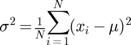
The variance can be calculated in a fast, single pass through the population, using the equivalent formula, below, which does not involve precalculating the population mean (Fig. 11.2).

By using the one-pass equation, after any number of data values have been processed, the running values of the average and variance can be easily determined; a handy trick, especially applicable to signal processing [8,9].

Section 11.3. The Dot Product, a Simple and Fast Correlation Method

Similarity scores are based on comparing one data object with another, attribute by attribute. Two similar variables will rise and fall together. A score can be calculated by summing the squares of the differences in magnitude for each attribute, and using the calculation to compute a final outcome, known as the correlation score. One of the most popular correlation methods is Pearson's correlation, which produces a score that can vary from − 1 to + 1. Two objects with a high score (near + 1) are highly similar [10]. Two uncorrelated objects would have a Pearson score near zero. Two objects that correlated inversely (i.e., one falling when the other rises) would have a Pearson score near − 1. [Glossary Correlation distance, Normalized compression distance, Mahalanobis distance]

The Pearson correlation for two objects, with paired attributes, sums the product of their differences from their object means and divides the sum by the product of the squared differences from the object means (Fig. 11.3).

Python's Scipy module offers a Pearson function. In addition to computing Pearson's correlation, the scipy function produces a two-tailed P-value, which provides some indication of the likelihood that two totally uncorrelated objects might produce a Pearson's correlation value as extreme as the calculated value. [Glossary P value, Scipy]

Let us look at a short python script, sci_pearson.py, that calculates the Pearson correlation on two lists.

from scipy.stats.stats import pearsonr
a = [1, 2, 3, 4]
b = [2, 4, 6, 8]
c = [1,4,6,9,15,55,62,-5]
d = [-2,-8,-9,-12,-80,14,15,2]
print("Correlation a with b: " + str(pearsonr(a,b)))
print("Correlation c with d: " + str(pearsonr(c,d)))

Here is the output of pearson.py

Correlation a with b: (1.0, 0.0)
Correlation c with d: (0.32893766587262174, 0.42628658412101167)

The Pearson correlation of a with b is 1 because the values of b are simply double the values of a; hence the values in a and b correlate perfectly with one another. The second number, “0.0”, is the calculated P value.

In the case of c correlated with d, the Pearson correlation, 0.329, is intermediate between 0 and 1, indicating some correlation. How does the Pearson correlation help us to simplify and reduce data? If two lists of data have a Pearson correlation of 1 or of − 1, this implies that one set of the data is redundant. We can assume the two lists have the same information content. If we were comparing two sets of data and found a Pearson correlation of zero, then we might assume that the two sets of data were uncorrelated, and that it would be futile to try to model (i.e., find a mathematical relationship for) the data. [Glossary Overfitting]

There are many different correlation measurements, and all of them are based on assumptions about how well-correlated sets of data ought to behave. A data analyst who works with gene sequences might impose a different set of requirements, for well-correlated data, than a data analyst who is investigating fluctuations in the stock market. Hence, there are many available correlation values that are available to data scientists, and these include: Pearson, Cosine, Spearman, Jaccard, Gini, Maximal Information Coefficient, and Complex Linear Pathway score. The computationally fastest of the correlation scores is the dot product (Fig. 11.4). In a recent paper comparing the performance of 12 correlation formulas the simple dot product led the pack [11].

Let us examine the various dot products that can be calculated for three sample vectors,

a = [1,4,6,9,15,55,62,-5]
b = [-2,-8,-9,-12,-80,14,15,2]
c = [2,8,12,18,30,110,124,-10]

Notice that vector c has twice the value of each paired attribute in vector a. We'll use the Python script, numpy_dot.py to compute the lengths of the vectors a, b, and c; and we will calculate the simple dot products, normalized by the product of the lengths of the vectors.

from __future__ import division
import numpy
from numpy import linalg
a = [1,4,6,9,15,55,62,-5]
b = [-2,-8,-9,-12,-80,14,15,2]
c = [2,8,12,18,30,110,124,-10]
a_length = linalg.norm(a)
b_length = linalg.norm(b)
c_length = linalg.norm(c)
print(numpy.dot(a,b) / (a_length ⁎ b_length))
print(numpy.dot(a,a) / (a_length ⁎ a_length))
print(numpy.dot(a,c) / (a_length ⁎ c_length))
print(numpy.dot(b,c) / (b_length ⁎ c_length))

Here is the commented output:

0.0409175385118 (Normalized dot product of a with b)
1.0        (Normalized dot product of a with a)
1.0        (Normalized dot product of a with c)
0.0409175385118 (Normalized dot product of b with c)

Inspecting the output, we see that the normalized dot product of a vector with itself is 1. The normalized dot product of a and c is also 1, because c is perfectly correlated with a, being twice its value, attribute by attribute. We also see that the normalized dot product of a and b is equal to the normalized dot product of b and c (0.0409175385118); because c is perfectly correlated with a and because dot products are transitive.

Section 11.4. Clustering

Clustering algorithms are currently very popular. They provide a way of taking a large set of data objects that seem to have no relationship to one another and to produce a visually simple collection of clusters wherein each cluster member is similar to every other member of the same cluster.

The algorithmic methods for clustering are simple. One of the most popular clustering algorithms is the k-means algorithm, which assigns any number of data objects to one of k clusters [12]. The number k of clusters is provided by the user. The algorithm is easy to describe and to understand, but the computational task of completing the algorithm can be difficult when the number of dimensions in the object (i.e., the number of attributes associated with the object), is large. [Glossary K-means algorithm, K-nearest neighbor algorithm]

Here is how the algorithm works for sets of quantitative data:

1. 1.  The program randomly chooses k objects from the collection of objects to be clustered. We will call each of these these k objects a focus.
2. 2.  For every object in the collection, the distance between the object and all of randomly chosen k objects (chosen in step 1) is computed.
3. 3.  A round of k-clusters are computed by assigning every object to its nearest focus.
4. 4.  The centroid focus for each of the k clusters is calculated. The centroid is the point that is closest to all of the objects within the cluster. Another way of saying this is that if you sum the distances between the centroid and all of the objects in the cluster, this summed distance will be smaller than the summed distance from any other point in space.
5. 5.  Steps 2, 3, and 4 are repeated, using the k centroid foci as the points for which all distances are computed.
6. 6.  Step 5 is repeated until the k centroid foci converge on a non-changing set of values (or until the program slows to an interminable crawl).

There are some serious drawbacks to the algorithm:

• –  The final set of clusters will sometimes depend on the initial, random choice of k data objects. This means that multiple runs of the algorithm may produce different outcomes.
• –  The algorithms are not guaranteed to succeed. Sometimes, the algorithm does not converge to a final, stable set of clusters.
• –  When the dimensionality is very high the distances between data objects (i.e., the square root of the sum of squares of the measured differences between corresponding attributes of two objects) can be ridiculously large and of no practical meaning. Computations may bog down, cease altogether, or produce meaningless results. In this case the only recourse may require eliminating some of the attributes (i.e., reducing dimensionality of the data objects). Subspace clustering is a method wherein clusters are found for computationally manageable subsets of attributes. If useful clusters are found using this method, additional attributes can be added to the mix to see if the clustering can be improved. [Glossary Curse of dimensionality]
• –  The clustering algorithm may succeed, producing a set of clusters of similar objects, but the clusters may have no practical value. They may miss important relationships among the objects, or they might group together objects whose similarities are totally non-informative.

At best, clustering algorithms should be considered a first step toward understanding how attributes account for the behavior of data objects.

Classifier algorithms are different from clustering algorithms. Classifiers assign a class (from a pre-existing classification) to an object whose class is unknown [12]. The k-nearest neighbor algorithm (not to be confused with the k-means clustering algorithm) is a simple and popular classifier algorithm. From a collection of data objects whose class is known, the algorithm computes the distances from the object of unknown class to the objects of known class. This involves a distance measurement from the feature set of the objects of unknown class to every object of known class (the test set). The distance measure uses the set of attributes that are associated with each object. After the distances are computed, the k classed objects with the smallest distance to the object of unknown class are collected. The most common class in the nearest k classed objects is assigned to the object of unknown class. If the chosen value of k is 1, then the object of unknown class is assigned the class of its closest classed object (i.e., the nearest neighbor).

The k-nearest neighbor algorithm is just one among many excellent classifier algorithms, and analysts have the luxury of choosing algorithms that match their data (e.g., sample size, dimensionality) and purposes [13]. Classifier algorithms differ fundamentally from clustering algorithms and from recommender algorithms in that they begin with an existing classification. Their task is very simple; assign an object to its proper class within the classification. Classifier algorithms carry the assumption that similarities among class objects determine class membership. This may not be the case. For example, a classifier algorithm might place cats into the class of small dogs because of the similarities among several attributes of cats and dogs (e.g., four legs, one tail, pointy ears, average weight about 8 pounds, furry, carnivorous, etc.). The similarities are impressive, but irrelevant. No matter how much you try to make it so, a cat is not a type of dog. The fundamental difference between grouping by similarity and grouping by relationship has been discussed in Section 5.1. [Glossary Recommender, Modeling]

Like clustering techniques, classifier techniques are computationally intensive when the dimension is high, and can produce misleading results when the attributes are noisy (i.e., contain randomly distributed attribute values) or non-informative (i.e., unrelated to correct class assignment).

Section 11.5. Methods for Data Persistence (Without Using a Database)

Your scripts create data objects, and the data objects hold data. Sometimes, these data objects are transient, existing only during a block or subroutine. At other times, the data objects produced by scripts represent prodigious amounts of data, resulting from complex and time-consuming calculations. What happens to these data structures when the script finishes executing? Ordinarily, when a script stops, all the data structures produced by the script simply vanish.

Persistence is the ability of data to outlive the program that produced it. The methods by which we create persistent data are sometimes referred to as marshalling or serializing. Some of the language specific methods are called by such colorful names as data dumping, pickling, freezing/thawing, and storable/retrieve. [Glossary Serializing, Marshalling, Persistence]

Data persistence can be ranked by level of sophistication. At the bottom is the exportation of data to a simple flat-file, wherein records are each one line in length, and each line of the record consists of a record key, followed by a list of record attributes. The simple spreadsheet stores data as tab delimited or comma separated line records. Flat-files can contain a limitless number of line records, but spreadsheets are limited by the number of records they can import and manage. Scripts can be written that parse through flat-files line by line (i.e., record by record), selecting data as they go. Software programs that write data to flat-files achieve a crude but serviceable type of data persistence.

A middle-level technique for creating persistent data is the venerable database. If nothing else, databases can create, store, and retrieve data records. Scripts that have access to a database can achieve persistence by creating database records that accommodate data objects. When the script ends, the database persists, and the data objects can be fetched and reconstructed for later use.

Perhaps the highest level of data persistence is achieved when complex data objects are saved in toto. Flat-files and databases may not be suited to storing complex data objects, holding encapsulated data values. Most languages provide built-in methods for storing complex objects, and a number of languages designed to describe complex forms of data have been developed. Data description languages, such as YAML (Yet Another Markup Language) and JSON (JavaScript Object Notation), can be adopted by any programming language.

Let us review some of the techniques for data persistence that are readily accessible to Python programmers.

Python pickles its data. Here, the Python script, pickle_up.py, pickles a string variable, in the save.p file.

import pickle
pumpkin_color = "orange"
pickle.dump( pumpkin_color, open("save.p","wb"))

The Python script, pickle_down.py, loads the pickled data, from the “save.p” file, and prints it to the screen.

import pickle
pumpkin_color = pickle.load(open("save.p","rb"))
print(pumpkin_color)

The output of the pickle_down.py script is shown here:

orange

Python has several database modules that will insert database objects into external files that persist after the script has executed. The database objects can be quickly called from the external module, with a simple command syntax [10]. Here is the Python script, lucy.py, that creates a tiny external database, using Python's most generic dbm.dumb module.

import dbm.dumb
lucy_hash = dbm.dumb.open('lucy', 'c')
lucy_hash["Fred Mertz"] = "Neighbor"
lucy_hash["Ethel Mertz"] = "Neighbor"
lucy_hash["Lucy Ricardo"] = "Star"
lucy_hash["Ricky Ricardo"] = "Band leader"
lucy_hash.close()

Here is the Python script, lucy_untie.py, that reads all of the key/value pairs held in the persistent database created for the lucy_hash dictionary object.

import dbm.dumb
lucy_hash = dbm.dumb.open('lucy')
for character in lucy_hash.keys():
 print(character.decode('utf-8') + " " + lucy_hash[character].decode('utf-8'))
lucy_hash.close()

Here is the output produced by the Python script, lucy_untie.py script.

Ethel Mertz Neighbor
Lucy Ricardo Star
Ricky Ricardo Band leader
Fred Mertz Neighbor

Persistence is a simple and fundamental process ensuring that data created in your scripts can be recalled by yourself or by others who need to verify your results. Regardless of the programming language you use, or the data structures you prefer, you will need to familiarize with at least one data persistence technique.

Section 11.6. Case Study: Climbing a Classification

Classifications are characterized by a linear ascension through a hierarchy. The parental classes of any instance of the classification can be traced as a simple, non-branched, and non-recursive, ordered, and uninterrupted list of ancestral classes.

In a prior work [10], I described how a large, publicly available, taxonomy data file could be instantly queried to retrieve any listed organism, and to compute its complete class lineage, back to the “root” class, the primordial origin the classification of living organisms [10]. Basically, the trick to climbing backwards up the class lineage involves building two dictionary objects, also known as associative arrays. One dictionary object (which we will be calling “namehash”) is composed of key/value pairs wherein each key is the identifier code of a class (in the nomenclature of the taxonomy data file), and each value is its name or label. The second dictionary object (which we'll be calling “parenthash”) is composed of key/value pairs wherein each key is the identifier code of a class, and each value is the identifier code of the parent class. Once you have prepared the namehash dictionary and the parenthash dictionary the entire ancestral lineage of every one of the many thousands of organisms included in the taxonomy of living species (contained in the taxonomy.dat file) can be reconstructed with just a few lines of Python code, as shown here:

for i in range(30):
   if id_name in namehash:
    outtext.write(namehash[id_name] + "
")
   if id_name in parenthash:
    id_name = parenthash[id_name]

The parts of the script that build the dictionary objects are left as an exercise for the reader. As an example of the script's output, here is the lineage for the Myxococcus bacteria:

Myxococcus
Myxococcaceae
Cystobacterineae
Myxococcales
Deltaproteobacteria
delta/epsilon subdivisions
Proteobacteria
Bacteria
cellular organisms
root

The words in this lineage may seem strange to laypersons, but taxonomists who view this lineage instantly grasp the place of organism within the classification of all living organisms. Every large and complex knowledge domain should have its own taxonomy, complete with a parent class for every child class. The basic approach to reconstructing lineages from the raw taxonomy file would apply to every field of study. For those interested in the taxonomy of living organisms, possibly the best documented classification of any kind, the taxonomy.dat file (exceeding 350 Mbytes) is available at no cost via ftp at:

• ftp://ftp.ebi.ac.uk/pub/databases/taxonomy/

Section 11.7. Case Study (Advanced): A Database Example

For industrial strength persistence, providing storage for millions or billions of data objects, database applications are a good choice. SQL (Systems Query Language, pronounced like “sequel”) is a specialized language used to query relational databases. SQL allows programmers to connect with large, complex server-based network databases. A high level of expertise is needed to install and implement the software that creates server-based relational databases responding to multi-user client-based SQL queries. Fortunately, Python provides access to SQLite, a free, and widely available spin-off of SQL [10]. The source code for SQLite is public domain. [Glossary Public domain]

SQLite is bundled into the newer distributions of Python, and can be called from Python scripts with an “import sqlite3” command. Here is a Python script, sqlite.py, that reads a very short dictionary into an SQL database.

import sqlite3, itertools
from sqlite3 import dbapi2 as sqlite
import string, re, os
mesh_hash = {}
entry = ()
mesh_hash["Fred Mertz"] = "Neighbor"
mesh_hash["Ethel Mertz"] = "Neighbor"
mesh_hash["Lucy Ricardo"] = "Star"
mesh_hash["Ricky Ricardo"] = "Band leader"
con = sqlite.connect('test1.db')
cur = con.cursor()
cur.executescript("""
  create table lucytable
  (
    name   varchar(64),
    term   varchar(64)
  );
  """)
for key,value in mesh_hash.items():
 entry = (key, value)
 cur.execute("insert into lucytable (name, term) values (?, ?)", entry)
con.commit()

Once created, entries in the SQL database file, test1.db, can be retrieved, as shown in the Python script, sqlite_read.py:

import sqlite3
from sqlite3 import dbapi2 as sqlite
import string, re, os
con = sqlite.connect('test1.db')
cur = con.cursor()
cur.execute("select ⁎ from lucytable")
for row in cur:
 print(row[0], row[1])

Here is the output of the sqlite_read.py script

Fred Mertz Neighbor
Ethel Mertz Neighbor
Lucy Ricardo Star
Ricky Ricardo Band leader

Databases, such as SQLite, are a great way to achieve data persistence, if you are adept at programming in SQL, and if you need to store millions of simple data objects. You may be surprised to learn that built-in persistence methods native to your favorite programming language may provide a simpler, more flexible option than proprietary database applications, when dealing with Big Data.

Section 11.8. Case Study (Advanced): NoSQL

Triples are the basic commodities of information science. Every triple represents a meaningful assertion, and collections of triples can be automatically integrated with other triples. As such all the triples that share the same identifier can be collected to yield all the available information that pertains to the unique object. Furthermore, all the triples that pertain to all the members of a class of objects can be combined to provide information about the class, and to find relationships among different classes of objects. This being the case, it should come as no surprise that databases have been designed to utilize triples as their data structure; dedicating their principal functionality to the creation, storage, and retrieval of triples.

Triple databases, also known as triplestores, are specialized variants of the better-known NoSQL databases; databases that are designed to store records consisting of nothing more than a key and value. In the case of triplestores, the key is the identifier of a data object, and the value is a metadata/data pair belonging associated with the identifier belonging to the data object.

Today, large triplestores exist, holding trillions of triples. At the current time, software development for triplestore databases is in a state of volatility. Triplestore databases are dropping in an out of existence, changing their names, being incorporated into other systems, or being redesigned from the ground up.

At the risk of showing my own personal bias, as an unapologetic Mumps fan, I would suggest that readers may want to investigate the value of using native Mumps as a triplestore database. Mumps, also known as the M programming language, is one of a small handful of ANSI-standard (American National Standard Institute) languages that includes C, Ada, and Fortran. It was developed in the 1960s and is still in use, primarily in hospital information systems and large production facilities [14]. The simple, hierarchical database design of Mumps lost favor through the last decades of the twentieth century, as relational databases gained popularity. In the past decade, with the push toward NoSQL databases holding massive sets of simplified data, Mumps has received renewed interest. As it happens, Mumps can be implemented as a powerful and high performance Triplestore database.

Versions of Mumps are available as open source, free distributions [15,16]. but the Mumps installation process can be challenging for those who are unfamiliar with the Mumps environment. Stalwarts who successfully navigate the Mumps installation process may find that Mumps' native features render it suitable for storing triples and exploring their relationships [17].

Glossary

AES The Advanced Encryption Standard (AES) is the cryptographic standard endorsed by the United States government as a replacement for the old government standard, DES (Data Encryption Standard). AES was chosen from among many different encryption protocols submitted in a cryptographic contest conducted by the United States National Institute of Standards and Technology, in 2001. AES is also known as Rijndael, after its developer. It is a symmetric encryption standard, meaning that the same password used for encryption is also used for decryption.

Associative array A data structure consisting of an unordered list of key/value data pairs. Also known as hash, hash table, map, symbol table, dictionary, or dictionary array. The proliferation of synonyms suggests that associative arrays, or their computational equivalents, have great utility. Associative arrays are used in Perl, Python, Ruby and most modern programming languages.

Black box In physics, a black box is a device with observable inputs and outputs, but what goes on inside the box is unknowable. The term is used to describe software, algorithms, machines, and systems whose inner workings are inscrutable.

Correlation distance Also known as correlation score. The correlation distance provides a measure of similarity between two variables. Two similar variables will rise rise and fall together [18,19]. The Pearson correlation score is popular, and can be easily implemented [10,20]. It produces a score that varies from − 1 to 1. A score of 1 indicates perfect correlation; a score of − 1 indicates perfect anti-correlation (i.e., one variable rises while the other falls). A Pearson score of 0 indicates lack of correlation. Other correlation measures can be applied to Big Data sets [18,19].

Curse of dimensionality As the number of attributes for a data object increases, the distance between data objects grows to enormous size. The multidimensional space becomes sparsely populated, and the distances between any two objects, even the two closest neighbors, becomes absurdly large. When you have thousands of dimensions, the space that holds the objects is so large that distances between objects become difficult or impossible to compute, and computational products become useless for most purposes.

K-means algorithm The k-means algorithm assigns any number of data objects to one of k clusters [12]. The algorithm is described fully in Chapter 9. The k-means algorithm should not be confused with the k-nearest neighbor algorithm.

K-nearest neighbor algorithm The k-nearest neighbor algorithm is a simple and popular classifier algorithm. From a collection of data objects whose class is known, the algorithm computes the distances from the object of unknown class to the objects of known class. This involves a distance measurement from the feature set of the objects of unknown class to every object of known class (the test set). After the distances are computed, the k classed objects with the smallest distance to the object of unknown class are collected. The most common class (i.e., the class with the most objects) among the nearest k classed objects is assigned to the object of unknown class. If the chosen value of k is 1, then the object of unknown class is assigned the class of its closest classed object (i.e., the nearest neighbor).

Mahalanobis distance A distance measure based on correlations between variables; hence, it measures the similarity of the objects whose attributes are compared. As a correlation measure, it is not influenced by the relative scale of the different attributes. It is used routinely in clustering and classifier algorithms.

Marshalling Marshalling, like serializing, is a method for achieving data persistence (i.e., saving variables and other data structures produced in a program, after the program has stopped running). Marshalling methods preserve data objects, with their encapsulated data and data structures.

Modeling Modeling involves explaining the behavior of a system, often with a formula, sometimes with descriptive language. The formula for the data describes the distribution of the data and often predicts how the different variables will change with one another. Consequently, modeling often provides reasonable hypotheses to explain how the data objects within a system will influence one another. Many of the great milestones in the physical sciences have arisen from a bit of data modeling supplemented by scientific genius (e.g., Newton's laws of mechanics and optics, Kepler's laws of planetary orbits, Quantum mechanics). The occasional ability to relate observation with causality endows modeling with greater versatility and greater scientific impact than the predictive techniques (e.g., recommenders, classifiers and clustering methods). Unlike the methods of predictive analytics, which tend to rest on a few basic assumptions about measuring similarities among data objects, the methods of data modeling are selected from every field of mathematics and are based on an intuitive approach to data analysis. In many cases, the modeler simply plots the data and looks for familiar shapes and patterns that suggest a particular type of function (e.g., logarithmic, linear, normal, Fourier series, Power law).

Normalized compression distance String compression algorithms (e.g., zip, gzip, bunzip) should yield better compression from a concatenation of two similar strings than from a concatenation of two highly dissimilar strings. The reason being that the same string patterns that are employed to compress a string (i.e., repeated runs of a particular pattern) are likely to be found in another, similar string. If two strings are completely dissimilar, then the compression algorithm would fail to find repeated patterns that enhance compressibility. The normalized compression distance is a similarity measure based on the enhanced compressibility of concatenated strings of high similarity [21]. A full discussion, with examples, is found in the Open Source Tools section of Chapter 4.

Overfitting Overfitting occurs when a formula describes a set of data very closely, but does not lead to any sensible explanation for the behavior of the data, and does not predict the behavior of comparable data sets. In the case of overfitting the formula is said to describe the noise of the system rather than the characteristic behavior of the system. Overfitting occurs frequently with models that perform iterative approximations on training data, coming closer and closer to the training data set with each iteration. Neural networks are an example of a data modeling strategy that is prone to overfitting.

P value The P value is the probability of getting a set of results that are as extreme or more extreme as the set of results you observed, assuming that the null hypothesis is true (that there is no statistical difference between the results). The P-value has come under great criticism over the decades, with a growing consensus that the P-value is often misinterpreted, used incorrectly, or used in situations wherein it does not apply [22]. In the realm of Big Data, repeated samplings of data from large data sets will produce small P-values that cannot be directly applied to determining statistical significance. It is best to think of the P-value as just another piece of information that tells you something about how sets of observations compare with one another; and not as a test of statistical significance.

Persistence Persistence is the ability of data to remain available in memory or storage after the program in which the data was created has stopped executing. Databases are designed to achieve persistence. When the database application is turned off, the data remains available to the database application when it is re-started at some later time.

Pseudorandom number generator It is impossible for computers to produce an endless collection of truly random numbers. Eventually, algorithms will cycle through their available variations and begins to repeat themselves, producing the same set of “random” numbers, in the same order; a phenomenon referred to as the generator's period. Because algorithms that produce seemingly random numbers are imperfect, they are known as pseudorandom number generators. The Mersenne Twister algorithm, which has an extremely long period, is used as the default random number generator in Python. This algorithm performs well on most of the tests that mathematicians have devised to test randomness.

Public domain Data that is not owned by an entity. Public domain materials include documents whose copyright terms have expired, materials produced by the federal government, materials that contain no creative content (i.e., materials that cannot be copyrighted), or materials donated to the public domain by the entity that holds copyright. Public domain data can be accessed, copied, and re-distributed without violating piracy laws. It is important to note that plagiarism laws and rules of ethics apply to public domain data. You must properly attribute authorship to public domain documents. If you fail to attribute authorship or if you purposefully and falsely attribute authorship to the wrong person (e.g., yourself), then this would be an unethical act and an act of plagiarism.

Recommender A collection of methods for predicting the preferences of individuals. Recommender methods often rely on one or two simple assumptions: (1) If an individual expresses a preference for a certain type of product, and the individual encounters a new product that is similar to a previously preferred product, then he is likely to prefer the new product; (2) If an individual expresses preferences that are similar to the preferences expressed by a cluster of individuals, and if the members of the cluster prefer a product that the individual has not yet encountered, then the individual will most likely prefer the product.

RegEx Short for Regular Expressions, RegEx is a syntax for describing patterns in text. For example, if I wanted to pull all lines from a text file that began with an uppercase “B” and contained at least one integer, and ended with the a lowercase x, then I might use the regular expression: “ˆB.⁎[0-9].⁎x$”. This syntax for expressing patterns of strings that can be matched by pre-built methods available to a programming language is somewhat standardized. This means that a RegEx expression in Perl will match the same pattern in Python, or Ruby, or any language that employs RegEx. The relevance of Regex to Big Data is several-fold. Regex can be used to build or transform data from one format to another; hence creating or merging data records. It can be used to convert sets of data to a desired format; hence transforming data sets. It can be used to extract records that meet a set of characteristics specified by a user; thus filtering subsets of data or executing data queries over text-based files or text-based indexes. The big drawback to using RegEx is speed: operations that call for many Regex operations, particularly when those operations are repeated for each parsed line or record, will reduce software performance. Regex-heavy programs that operate just fine on megabyte files may take hours, days or months to parse through terabytes of data.
A 12-line python script, file_search.py, prompts the user for the name of a text file to be searched, and then prompts the user to supply a RegEx pattern. The script will parse the text file, line by line, displaying those lines that contain a match to the RegEx pattern.
import sys, string, re
print("What is file would you like to search?")
filename = sys.stdin.readline()
filename = filename.rstrip()
print("Enter a word, phrase or regular expression to search.")
word_to_search = (sys.stdin.readline()).rstrip()
infile = open (filename, "r")
regex_object = re.compile(word_to_search, re.I)
for line in infile:
     m = regex_object.search(line)
     if m:
           print(line)

Scipy Scipy, like numpy, is an open source extension to Python [23]. It includes many very useful mathematical routines commonly used by scientists, including: integration, interpolation, Fourier transforms, signal processing, linear algebra, and statistics. Scipy can be downloaded as a suite of modules from: http://www.scipy.org/scipylib/download.html. You can spare yourself the trouble of downloading individual installations of numpy and scipy by downloading Anaconda, a free distribution that bundles hundreds of python packages, along with a recent version of Python. Anaconda is available at: https://store.continuum.io/cshop/anaconda/

Serializing Serializing is a plesionym (i.e., near-synonym) for marshalling and is a method for taking data produced within a script or program, and preserving it in an external file, that can be saved when the program stops, and quickly reconstituted as needed, in the same program or in different programs. The difference, in terms of common usage, between serialization and marshalling is that serialization usually involves capturing parameters (i.e., particular pieces of information), while marshalling preserves all of the specifics of a data object, including its structure, content, and code content). As you might imagine, the meaning of terms might change depending on the programming language and the intent of the serializing and marshalling methods.

System call Refers to a command, within a running script, that calls the operating system into action, momentarily bypassing the programming interpreter for the script. A system call can do essentially anything the operating system can do via a command line.

Undifferentiated software Intellectual property disputes have driven developers to divide software into two categories: undifferentiated software and differentiated software. Undifferentiated software comprises the fundamental algorithms that everyone uses whenever they develop a new software application. It is in nobody's interest to assign patents to basic algorithms and their implementations. Nobody wants to devote their careers to prosecuting or defending tenuous legal claims over the ownership of the fundamental building blocks of computer science. Differentiated software comprises customized applications that are sufficiently new and different from any preceding product that patent protection would be reasonable.