4 Local differential privacy for machine learning

This chapter covers

• Local differential privacy (LDP)
• Implementing the randomized response mechanism for LDP
• LDP mechanisms for one-dimensional data frequency estimation
• Implementing and experimenting with different LDP mechanisms for one-dimensional data

In the previous two chapters we discussed centralized differential privacy (DP), where there is a trusted data curator who collects data from individuals and applies different techniques to obtain differentially private statistics about the population. Then the curator publishes privacy-preserving statistics about this population. However, these techniques are unsuitable when individuals do not completely trust the data curator. Hence, various techniques to satisfy DP in the local setting have been studied to eliminate the need for a trusted data curator. In this chapter we will walk through the concept, mechanisms, and applications of the local version of DP, local differential privacy (LDP).

This chapter will mainly look at how LDP can be implemented in ML algorithms by looking at different examples and implementation code. In the next chapter we’ll also walk you through a case study of applying LDP naive Bayes classification for real-world datasets.

4.1 What is local differential privacy?

DP is a widely accepted standard for quantifying individual privacy. In the original definition of DP, there is a trusted data curator who collects data from individuals and applies techniques to obtain differentially private statistics. This data curator then publishes privacy-preserving statistics about the population. We looked at how to satisfy DP in the context of ML in chapters 2 and 3. However, those techniques cannot be applied when individuals do not completely trust the data curator.

Different techniques have been proposed to ensure DP in the local setting without a trusted data curator. In LDP, individuals send their data to the data aggregator after privatizing the data by perturbation (see figure 4.1). These techniques provide plausible deniability for individuals. The data aggregator collects all the perturbed values and makes an estimation of the statistics, such as the frequency of each value in the population.

Figure 4.1 Centralized vs. local DP

4.1.1 The concept of local differential privacy

Many real-world applications, including those from Google and Apple, have adopted LDP. Before we discuss the concept of LDP and how it works, let’s look at how it’s applied to real-world products.

How Google and Apple use LDP

In 2014 Google introduced Randomized Aggregatable Privacy-Preserving Ordinal Response (RAPPOR) [1], a technology for anonymously crowdsourcing statistics from end-user client software with strong privacy guarantees. This technology has lately been integrated with the Chrome web browser. Over the last five years, RAPPOR has processed up to billions of daily, randomized reports in a manner that guarantees LDP. The technology is designed to collect statistics on client-side values and strings over large numbers of clients, such as categories, frequencies, histograms, and other statistics. For any reported value, RAPPOR offers a strong deniability guarantee for the reporting client, which strictly limits the private information disclosed, as measured by DP, and it even holds for a single client that often reports on the same value.

In 2017 Apple also released a research paper on how it uses LDP to improve the user experience with their products by getting insight into what many of their users are doing. For example, what new words are trending and might make the most relevant suggestions? What websites have problems that could affect battery life? Which emojis are chosen most often? The DP technology used by Apple is rooted in the idea that slightly biased statistical noise can mask a user’s data before it is shared with Apple. If many people submit the same data, the noise added can average out over large numbers of data points, and Apple can see meaningful information emerge. Apple details two techniques for collecting data while protecting users’ privacy: the Count Mean Sketch and the Hadamard Count Mean Sketch. Both approaches insert random information into the data being collected. That random information effectively obfuscates any identifying aspects of the data so that it cannot be traced back to individuals.

As you can see in these examples, LDP is usually being applied for mean or frequency estimation. Frequency estimation in a survey (or in survey-like problems) is one of the most common approaches to utilizing LDP in day-to-day applications. For instance, companies, organizations, and researchers often use surveys to analyze behavior or assess thoughts and opinions, but collecting information from individuals for research purposes is challenging due to privacy reasons. Individuals may not trust the data collector to not share sensitive or private information. And although an individual may participate in a survey anonymously, it can sometimes still be possible to identify the person by using the information provided. On the other hand, even though the people conducting the surveys are more interested in the distribution of the survey answers, rather than the information about specific individuals, it is quite difficult for them to earn the trust of survey participants when it comes to sensitive information. This is where LDP comes in.

LDP in detail

Now that you have some background on how LDP is used, let’s look at the details. LDP is a way of measuring individual privacy when the data collector is not trusted. LDP aims to guarantee that when an individual provides a value, it should be challenging to identify the original value, which provides the privacy protection. Many LDP mechanisms also aim to estimate the distribution of the population as accurately as possible based on the aggregation of the perturbed data collected from all individuals.

Figure 4.2 illustrates the typical use of LDP. First, each individual (data owner) generates or collects their own data, such as survey answers or personal data. Then, each individual perturbs their data locally using a specific LDP mechanism (which we’ll discuss in section 4.2). After conducting the perturbation, each individual sends their data to a data collector, who will perform the data aggregation and statistics or models estimation. Finally, the estimated statistics or models will be published. It would be extremely hard for adversaries to infer an individual’s data based on such published information (as guaranteed by the definition of LDP).

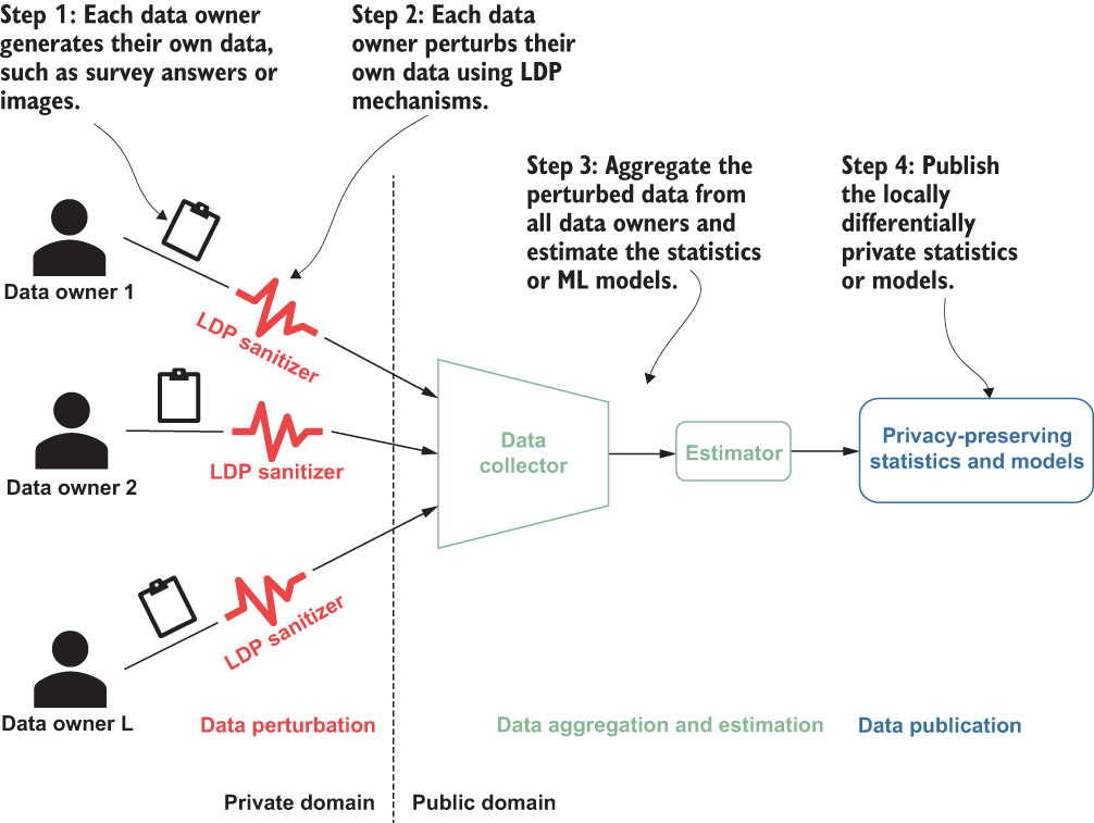
Figure 4.2 How local differential privacy works

LDP states that for any published estimated statistics or models using an ϵ-LDP mechanism, the probability of distinguishing two input values (i.e., an individual’s data) by the data collector (or any other adversaries in the public domain) is at most e^-ϵ.

A protocol P satisfies ϵ-LDP if for any two input values v₁ and v₂ and any output o in the output space of P, we have

where Pr[⋅] means probabilities. Pr[P(v₁) = o] is the probability that given input v₁ to P, it outputs o. The ϵ parameter in the definition is the privacy parameter or the privacy budget. It helps to tune the amount of privacy the definition provides. Small values of ϵ require P to provide very similar outputs when given similar inputs and therefore provide higher levels of privacy; large values of ϵ allow less similarity in the outputs and therefore provide less privacy. For instance, as shown in figure 4.3, for a small value of ϵ, given a perturbed value o, it is (almost) equally likely that o resulted from any input value, that is, v₁ or v₂. In this way, just by observing an output, it is hard to infer back to its corresponding input; hence, the privacy of the data is ensured.

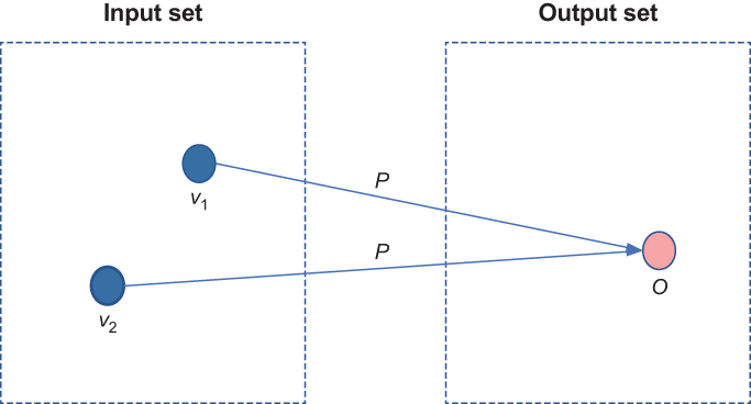
Figure 4.3 How ϵ-LDP works. Given a perturbed value o, it is (almost) equally likely that it resulted from any input value—either v₁ or v₂ in this example.

We have now discussed the concept and definition of LDP and looked at how it differs from centralized DP. Before we introduce any of the LDP mechanisms, let’s look at a scenario where we’ll apply LDP.

An LDP scenario with a survey

Answering questions in online surveys or social network quizzes via tools like SurveyMonkey is a widespread practice today. LDP can protect the answers of these surveys before they leave the data owners. Throughout this chapter, we will use the following scenario to demonstrate the design and implementation of LDP mechanisms.

Let’s say company A wants to determine the distribution of its customers (for a targeted advertising campaign). It conducts a survey, and sample survey questions might look like these:

• Are you married?

• What is your occupation?

• How old are you?

• What is your race category?

However, these questions are highly sensitive and private. To encourage its customers to participate in the survey, company A should provide privacy guarantees while still keeping the estimated distribution of its customers as accurate as possible when conducting the survey.

Not surprisingly, LDP is one technique that could help the company. There are several different LDP mechanisms that deal with different scenarios (i.e., data type, data dimensions, etc.). For instance, the answer to the question “Are you married?” is simply a categorical binary result: “yes” or “no.” A randomized response mechanism would be suitable to solve such scenarios. On the other hand, the answers to the questions “What is your occupation?” and “What is your race category?” are still categorical but would be single items from a set of possible answers. For such scenarios, direct encoding and unary encoding mechanisms would work better. Moreover, for questions like “What is your age?” the answer is numerical, and the summary of all the answers looks like a histogram. We can use histogram encoding in such cases.

Given that simple outline of how LDP can be used in practice, we will introduce how LDP works in real-world scenarios by walking through how we could design and implement solutions that apply different LDP mechanisms for diverse survey questions. We will start with the most straightforward LDP mechanism, the randomized response.

4.1.2 Randomized response for local differential privacy

As discussed in chapter 2, randomized response (binary mechanism) is one of the oldest and simplest DP mechanisms, but it also satisfies LDP. In this section you will learn how to use the randomized response to design and implement an LDP solution for a privacy-preserving binary survey.

Let’s assume we want to survey a group of people to determine the number of people more than 50 years old. Each individual will be asked, “Are you more than 50 years old?” The answer collected from each individual will be either “yes” or “no.” The answer is considered a binary response to the survey question, where we give a binary value of 1 to each “yes” answer and a binary value of 0 to each “no” answer. Thus, the final goal is to determine the number of people who are more than 50 years old by counting the number of 1s sent by the individuals as their answers. How can we use the randomized response mechanism to design and implement a locally differentially private survey to gather the answers to this simple “yes” or “no” question?

Here comes the privacy protection. As shown in listing 4.1, each individual will either respond with the true answer or provide a randomized response according to the algorithm. Thus, the privacy of the individuals will be well protected. Also, since each individual will provide the actual answer with a probability of 0.75 (i.e., 1/2 + 1/4 = 0.75) and give the wrong answer with a probability of 0.25, more individuals will provide true answers. Therefore, we will retain enough essential information to estimate the distribution of the population’s statistics (i.e., the number of individuals more than 50 years old).

Listing 4.1 Randomized response-based algorithm

def random_response_ages_adult(response):
    true_ans = response > 50

    if np.random.randint(0, 2) == 0:            ❶
        return true_ans                         ❷
    else:
        return np.random.randint(0, 2) == 0     ❸

❶ Flip the first coin.

❷ Return the true answer.

❸ Flip the second coin and return the randomized answer.

Let’s implement and test our algorithm on the US Census dataset as shown in listing 4.2. In the next section, we will discuss more practical use cases, but for now we will use the census dataset to demonstrate how you can estimate the aggregated values.

Listing 4.2 Playing with the US Census dataset

import numpy as np
import matplotlib.pyplot as plt

ages_adult = np.loadtxt("https://archive.ics.uci.edu/ml/machine-
➥ learning-databases/adult/adult.data", usecols=0, delimiter=", ")

total_count = len([i for i in ages_adult]) 
age_over_50_count= len([i for i in ages_adult if i > 50]) 

print(total_count)
print(age_over_50_count)
print(total_count-age_over_50_count)

The output will be as follows:

32561
6460
26101

As you can see, there are 32,561 individuals in the US Census dataset: 6,460 individuals are more than 50 years old, and 26,101 individuals are younger than or equal to 50 years old.

Now let’s see what will happen if we apply our randomized response-based algorithm to the same application.

Listing 4.3 Data perturbation

perturbed_age_over_50_count = len([i for i in ages_adult 
➥ if random_response_ages_adult(i)]) 
print(perturbed_age_over_50_count)
print(total_count-perturbed_age_over_50_count)

The result will be as follows:

11424
21137

As you can see, after applying our randomized response algorithm, the perturbed number of individuals more than 50 years old becomes 11,424, and the perturbed number of individuals younger than or equal to 50 years old is 21,137. In this result, the number of people over 50 is still less than those below or equal to 50, which is in line with the trend of the original dataset. However, this result, 11,424, seems a bit away from the actual result that we want to estimate, 6,460.

Now the question is how to estimate the actual number of people over 50 years old based on our randomized response-based algorithm and the results we’ve got so far. Apparently, directly using the number of 1 or “yes” values is not a precise estimation of the actual values.

To precisely estimate the actual value of the number of people more than 50 years old, we should consider the source of the randomness in our randomized response-based algorithm and estimate the number of 1s that are from the people who are actually older than 50 years, and the number of 1s that are from the randomized response results. In our algorithm, each individual will tell the truth with a probability of 0.5 and make a random response again with a probability of 0.5. Each random response will result in a 1 or “yes” with a probability of 0.5. Thus, the probability that an individual replies 1 or “yes” solely based on randomness (rather than because they are actually older than 50 years) is 0.5 × 0.5 = 0.25. Therefore, as you can see, 25% of our total 1 or “yes” values are false yesses.

On the other hand, due to the first flip of the coin, we split the people who were telling the truth and those who were giving answers randomly. In other words, we can assume there are around the same number of people older than 50 in both groups. Therefore, the number of people over 50 years old is roughly twice the number of people over 50 years old in the group of people who were telling the truth.

Now that we know the problem, we can use the following implementation to estimate the total number of people over 50 years old.

Listing 4.4 Data aggregation and estimation

answers = [True if random_response_ages_adult(i) else False 
➥ for i in ages_adult ]                                       ❶

def random_response_aggregation_and_estimation(answers):       ❷
    false_yesses = len(answers)/4                              ❸

    total_yesses = np.sum([1 if r else 0 for r in answers])    ❹

    true_yesses = total_yesses - false_yesses                  ❺

    rr_result = true_yesses*2                                  ❻
    return rr_result

estimated_age_over_50_count = 
➥ random_response_aggregation_and_estimation(answers)
print(int(estimated_age_over_50_count))
print(total_count-int(estimated_age_over_50_count))

❶ Perturbation

❷ Data aggregation and estimation

❸ One-quarter (0.25) of the answers are expected to be 1s or yesses coming from the random answers (false yesses resulting from coin flips).

❹ The total number of yesses received

❺ The number of true yesses is the difference between the total number of yesses and the false yesses.

❻ Because true yesses estimates the total number of yesses in the group that was telling the truth, the total number of yesses can be estimated as twice the true yesses.

You will get output like the following:

6599
25962

Now we have a much more precise estimation of the number of people over 50 years old. How close is the estimate? The relative error is just (6599 - 6460)/6460 = 2.15%. Our randomized response-based algorithm seems to have done a good job of estimating the number of people over 50 years old. Also, based on our analysis in chapter 2, the privacy budget of this algorithm is ln(3) (i.e., ln(3) ≈ 1.099). In other words, our algorithm satisfies ln(3)-LDP.

In this section we revisited the randomized response mechanism in the context of LDP by designing and implementing a privacy-preserving binary-question survey application. As you can see, the randomized response mechanism is only good at dealing with problems based on single binary questions, that is, “yes” or “no” questions.

In practice, most questions or tasks are not simply “yes” or “no” questions. They can involve choosing from a finite set of values (such as “What is your occupation?”) or returning a histogram of a dataset (such as the distribution of the age of a group of people). We need more general and advanced mechanisms to tackle such problems. In the next section we will introduce more common LDP mechanisms that can be used in more widespread and complex situations.

4.2 The mechanisms of local differential privacy

We’ve discussed the concept and definition of LDP and how it works using the randomized response mechanism. In this section we’ll discuss some commonly utilized LDP mechanisms that work in more general and complex scenarios. These mechanisms will also serve as the building blocks for LDP ML algorithms in the next chapter’s case study.

4.2.1 Direct encoding

The randomized response mechanism works for binary (yes or no) questions with LDP. But how about questions that have more than just two answers? For instance, what if we want to determine the number of people with each occupation within the US Census dataset? The occupations could be sales, engineering, financial, technical support, etc. A decent number of different algorithms have been proposed for solving this problem in the local model of differential privacy [2], [3], [4]. Here we’ll start with one of the simplest mechanisms, called direct encoding.

Given a problem where we need to utilize LDP, the first step is to define the domain of different answers. For example, if we want to learn how many people are in each occupation within the US Census dataset, the domain would be the set of professions available in the dataset. The following lists all the professions in the census dataset.

Listing 4.5 Number of people in each occupation domain

import pandas as pd
import numpy as np
import matplotlib.pyplot as plt
import sys
import io
import requests
import math

req = requests.get("https://archive.ics.uci.edu/ml/machine-learning-
➥ databases/adult/adult.data").content             ❶
adult = pd.read_csv(io.StringIO(req.decode('utf-8')), 
➥ header=None, na_values='?', delimiter=r", ")
adult.dropna()
adult.head()

domain = adult[6].dropna().unique()                 ❷
domain.sort()
domain

❶ Load data.

❷ The domains

The result will look like the following:

array(['Adm-clerical', 'Armed-Forces', 'Craft-repair', 'Exec-managerial',
       'Farming-fishing', 'Handlers-cleaners', 'Machine-op-inspct',
       'Other-service', 'Priv-house-serv', 'Prof-specialty',
       'Protective-serv', 'Sales', 'Tech-support', 'Transport-moving'],
      dtype=object)

As we discussed in the previous section, LDP mechanisms usually contain three functions: encoding, which encodes each answer; perturbation, which perturbs the encoded answers; and aggregation and estimation, which aggregates the perturbed answers and estimates the final results. Let’s define those three functions for the direct encoding mechanism.

In the direct encoding mechanism, there is usually no encoding of input values. We can use each input’s index in the domain set as its encoded value. For example, “Armed-Forces” is the second element of the domain, so the encoded value of “Armed-Forces” is 1 (the index starts from 0).

Listing 4.6 Applying direct encoding

def encoding(answer):
    return int(np.where(domain == answer)[0])

print(encoding('Armed-Forces'))     ❶
print(encoding('Craft-repair'))
print(encoding('Sales'))
print(encoding('Transport-moving'))

❶ Test the encoding.

The output of the listing 4.6 will be as follows:

1
2
11
13

As mentioned, “Armed-Forces” is assigned the value 1, “Craft-repair” is assigned the value 2, and so on.

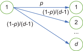
Figure 4.4 The perturbation of direct encoding

Our next step is the perturbation. Let’s review the perturbation of direct encoding (illustrated in figure 4.4). Each person reports their value v correctly with a probability of the following:

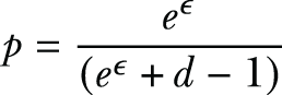
Or they report one of the remaining d - 1 values with a probability of

where d is the size of the domain set.

For instance, in our example, since there are 14 different professions listed in the US Census dataset, the size of the domain set is d = 14. As shown in listing 4.7, if we choose ϵ = 5.0, we have p = 0.92 and q = 0.0062, which will output the actual value with a higher probability. If we choose ϵ = 0.1, we have p = 0.078 and q = 0.071, which will generate the actual value with a much lower probability, thus providing more privacy guarantees.

Listing 4.7 Perturbation algorithm in direct encoding

def perturbation(encoded_ans, epsilon = 5.0):
    d = len(domain)                                           ❶
    p = pow(math.e, epsilon) / (d - 1 + pow(math.e, epsilon))
    q = (1.0 - p) / (d - 1.0)

    s1 = np.random.random()
    if s1 <= p:
        return domain[encoded_ans]                            ❷
    else:
        s2 = np.random.randint(0, d - 1)
        return domain[(encoded_ans + s2) % d]

print(perturbation(encoding('Armed-Forces')))                 ❸
print(perturbation(encoding('Craft-repair')))
print(perturbation(encoding('Sales')))
print(perturbation(encoding('Transport-moving')))
print()

print(perturbation(encoding('Armed-Forces'), epsilon = .1))   ❹
print(perturbation(encoding('Craft-repair'), epsilon = .1))
print(perturbation(encoding('Sales'), epsilon = .1))
print(perturbation(encoding('Transport-moving'), epsilon = .1))

❶ Size of the domain set

❷ Return itself with probability p

❸ Test the perturbation, epsilon = 5.0.

❹ Test the perturbation, epsilon = .1.

The output will look like the following:

Armed-Forces
Craft-repair
Sales
Transport-moving

Other-service
Handlers-cleaners
Farming-fishing
Machine-op-inspct

Let’s try to understand what is happening here. When you assign the epsilon value to be 5.0 (look at the first four results in the output), you get the actual values with a much higher probability. In this case, the accuracy is 100%. However, when you assign epsilon to be a much smaller number (in this case 0.1), the algorithm will generate actual values with a much lower probability; hence, the privacy assurance is better. As can be seen from the latter four results in the output, we are getting different occupations as a result. You can play with assigning different epsilon values in the code to see how it affects the final results.

Let’s see what would happen after applying the perturbation to the answers to the survey question, “What is your occupation?” as follows.

Listing 4.8 Results of direct encoding after perturbation

perturbed_answers = pd.DataFrame([perturbation(encoding(i)) 
➥ for i in adult_occupation])
perturbed_answers.value_counts().sort_index()

The result after applying the direct encoding will look like this:

Adm-clerical         3637
Armed-Forces          157
Craft-repair         3911
Exec-managerial      3931
Farming-fishing      1106
Handlers-cleaners    1419
Machine-op-inspct    2030
Other-service        3259
Priv-house-serv       285
Prof-specialty       4011
Protective-serv       741
Sales                3559
Tech-support         1021
Transport-moving     1651

Now that we have the perturbed results, let’s compare them with the actual results.

Listing 4.9 Comparison of actual results and perturbed values

adult_occupation = adult[6].dropna()         ❶
adult_occupation.value_counts().sort_index()

❶ The number of people in each occupation category

These are the actual results of the number of people in each occupation category:

Adm-clerical         3770
Armed-Forces            9
Craft-repair         4099
Exec-managerial      4066
Farming-fishing       994
Handlers-cleaners    1370
Machine-op-inspct    2002
Other-service        3295
Priv-house-serv       149
Prof-specialty       4140
Protective-serv       649
Sales                3650
Tech-support          928
Transport-moving     1597

For clarity, let’s compare the results side by side, as shown in table 4.1. As can be seen, some of the aggregations of the perturbed answers have very high errors compared to the actual values. For instance, for the number of people with the occupation “Armed-Forces,” the perturbed value is 157 but the true value is 9.

Table 4.1 Number of people in each profession, before and after perturbation

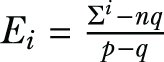
To overcome such errors, we need to have an aggregation and estimation function along with the direct encoding mechanism. In the aggregation and estimation, when the aggregator collects the perturbed values from n individuals, it estimates the frequency of each occupation I ∈ {1,2,...,d } as follows: First, c_i is the number of times i is reported. The estimated number of occurrences of value i in the population is computed as E_i = (c_i - n ⋅q)/(p - q). To ensure the estimated number is always a non-negative value, we set E_i = max(E_i, 1). You can try implementing listing 4.10 to see how it works.

Listing 4.10 Applying aggregation and estimation to direct encoding

def aggregation_and_estimation(answers, epsilon = 5.0):
    n = len(answers)
    d = len(domain)
    p = pow(math.e, epsilon) / (d - 1 + pow(math.e, epsilon))
    q = (1.0 - p) / (d - 1.0)

    aggregator = answers.value_counts().sort_index()
    
    return [max(int((i - n*q) / (p-q)), 1) for i in aggregator]  

estimated_answers = aggregation_and_estimation(perturbed_answers)    ❶
list(zip(domain, estimated_answers))

❶ Data aggregation and estimation

You will get something like the following as the output:

[('Adm-clerical', 3774),
 ('Armed-Forces', 1),
 ('Craft-repair', 4074),
 ('Exec-managerial', 4095),
 ('Farming-fishing', 1002),
 ('Handlers-cleaners', 1345),
 ('Machine-op-inspct', 2014),
 ('Other-service', 3360),
 ('Priv-house-serv', 103),
 ('Prof-specialty', 4183),
 ('Protective-serv', 602),
 ('Sales', 3688),
 ('Tech-support', 909),
 ('Transport-moving', 1599)]

With that result, let’s compare the estimated results to the actual results as shown in table 4.2. As you can see, the estimated results of the direct encoding mechanism are much more precise than the perturbed results when using the privacy budget x = 5.0. You can try changing the privacy budget in this code or apply the code to other datasets to see how it works.

Table 4.2 Number of people in each profession, before and after aggregation and estimation

You’ve now seen one LDP mechanism that uses direct encoding. Those steps can be summarized in the following three components:

• Encoding: Direct encoding (generalization of binary randomized response)

• Perturbation:  for ε-LDP

• Estimation:  where q = (1 - p)/(>d - 1)

4.2.2 Histogram encoding

The direct encoding mechanism enables us to apply LDP to categorical and discrete problems. In contrast, histogram encoding enables us to apply LDP to numerical and continuous data.

Consider a survey question that has numerical and continuous answers. For example, suppose someone wants to know the distribution or histogram of people’s ages within a group of people, which we cannot achieve with direct encoding. They could conduct a survey to ask each individual a survey question: “What is your age?” Let’s take the US Census dataset as an example and plot the histogram of people’s ages.

Listing 4.11 Plotting a histogram with people’s ages

import pandas as pd
import numpy as np
import matplotlib.pyplot as plt
import sys
import io
import requests
import math

req = requests.get("https://archive.ics.uci.edu/ml/machine-learning-
➥ databases/adult/adult.data").content                   ❶
adult = pd.read_csv(io.StringIO(req.decode('utf-8')), 
➥ header=None, na_values='?', delimiter=r", ")
adult.dropna()
adult.head()

adult_age = adult[0].dropna()                             ❷
ax = adult_age.plot.hist(bins=100, alpha=1.0)

❶ Load data.

❷ The ages of the people

The output will look like the histogram in figure 4.5, indicating the number of people in each age category. As you can see, the largest number of people are in the age ranges of ~20 to 40, whereas a lesser number of people are reported in the other values. The histogram-encoding mechanism is designed to deal with such numerical and continuous data.

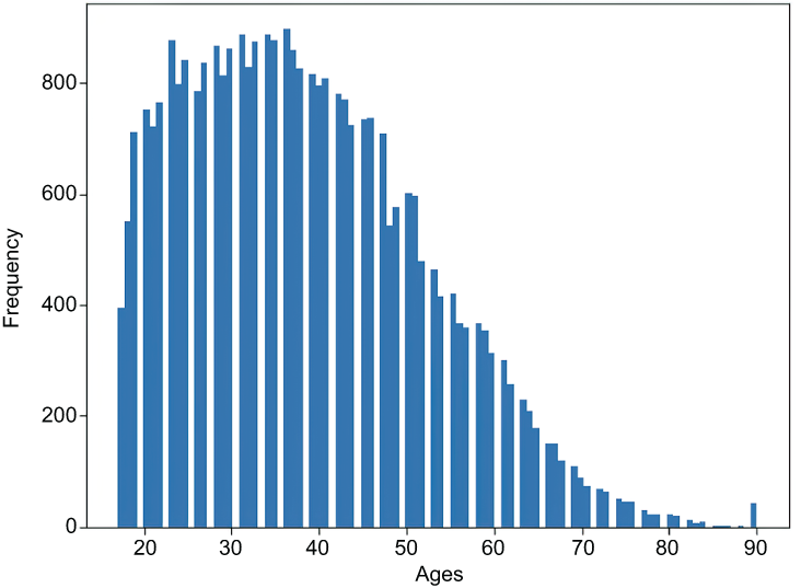
Figure 4.5 Histogram of people’s ages from US Census dataset

We first need to define the input domain (i.e., the survey answers). Here, we assume all the people taking the survey will be from 10 to 100 years old.

Listing 4.12 Input domain of the survey people’s ages

domain = np.arange(10, 101)    ❶
domain.sort()
domain

❶ The domain is in the range of 10 to 100.

Therefore, the domain will look like this:

array([ 10,  11,  12,  13,  14,  15,  16,  17,  18,  19,  20,  21,  22,
        23,  24,  25,  26,  27,  28,  29,  30,  31,  32,  33,  34,  35,
        36,  37,  38,  39,  40,  41,  42,  43,  44,  45,  46,  47,  48,
        49,  50,  51,  52,  53,  54,  55,  56,  57,  58,  59,  60,  61,
        62,  63,  64,  65,  66,  67,  68,  69,  70,  71,  72,  73,  74,
        75,  76,  77,  78,  79,  80,  81,  82,  83,  84,  85,  86,  87,
        88,  89,  90,  91,  92,  93,  94,  95,  96,  97,  98,  99, 100])

In histogram encoding, an individual encodes their value v as a length-d vector [0.0,0.0,...,0.0,1.0,0.0,...,0.0] where only the vth component is 1.0 and the remaining components are 0.0. For example, suppose there are 6 values in total ({1,2,3,4,5,6}), that is, d = 6, and the actual value to be encoded is 6. In that case, the histogram encoding will output the vector ({0.0,0.0,0.0,0.0,0.0,1.0}), where only the sixth position of the vector is 1.0 and all the other positions are 0.0 (see figure 4.6).

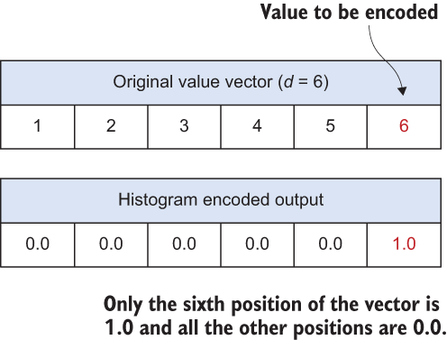
Figure 4.6 How histogram encoding works

The following listing shows the implementation of the encoding function.

Listing 4.13 Histogram encoding

def encoding(answer):
    return [1.0 if d == answer else 0.0 for d in domain]

print(encoding(11))                                           ❶

answers = np.sum([encoding(r) for r in adult_age], axis=0)    ❷
plt.bar(domain, answers)

❶ Test the encoding for input age 11.

❷ Data encoding plot

The output of listing 4.13 follows, and the histogram result is shown in figure 4.7:

[0.0, 1.0, 0.0, 0.0, 0.0, 0.0, 0.0, 0.0, 0.0, 0.0, 0.0, 0.0, 0.0, 0.0, 0.0, 0.0, 0.0, 0.0, 0.0, 0.0, 0.0, 0.0, 0.0, 0.0, 0.0, 0.0, 0.0, 0.0, 0.0, 0.0, 0.0, 0.0, 0.0, 0.0, 0.0, 0.0, 0.0, 0.0, 0.0, 0.0, 0.0, 0.0, 0.0, 0.0, 0.0, 0.0, 0.0, 0.0, 0.0, 0.0, 0.0, 0.0, 0.0, 0.0, 0.0, 0.0, 0.0, 0.0, 0.0, 0.0, 0.0, 0.0, 0.0, 0.0, 0.0, 0.0, 0.0, 0.0, 0.0, 0.0, 0.0, 0.0, 0.0, 0.0, 0.0, 0.0, 0.0, 0.0, 0.0, 0.0, 0.0, 0.0, 0.0, 0.0, 0.0, 0.0, 0.0, 0.0, 0.0, 0.0, 0.0]

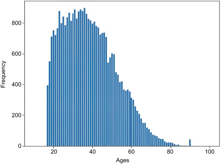
Figure 4.7 Histogram of encoded ages

The data owners perturb their value by adding Lap(2/ϵ) to each component in the encoded value, where Lap(2/ϵ) is a sample from the Laplace distribution with mean 0 and scale parameter 2/ϵ. If you need a refresher on the Laplace distribution and its properties, look back to section 2.1.2.

When the data aggregator collects all the perturbed values, the aggregator has two options for estimation methods:

• Summation with histogram encoding (SHE)

• Thresholding with histogram encoding (THE)

Summation with histogram encoding (SHE)

Summation with histogram encoding (SHE) calculates the sum of all values reported by individuals. To estimate the number of occurrences of value i in the population, the data aggregator sums the ith component of all reported values.

The following listing shows the implementation of the perturbation using SHE.

Listing 4.14 Summation with histogram encoding

def she_perturbation(encoded_ans, epsilon = 5.0):
    return [she_perturb_bit(b, epsilon) for b in encoded_ans]

def she_perturb_bit(bit, epsilon = 5.0):
    return bit + np.random.laplace(loc=0, scale = 2 / epsilon)

print(she_perturbation(encoding(11)))                         ❶
print()

print(she_perturbation(encoding(11), epsilon = .1))           ❷

she_estimated_answers = np.sum([she_perturbation(encoding(r)) 
➥ for r in adult_age], axis=0)                               ❸
plt.bar(domain, she_estimated_answers)

❶ Test the perturbation, epsilon = 5.0.

❷ Test the perturbation, epsilon = .1.

❸ Data perturbation, aggregation, and estimation

The output of listing 4.14 follows, and figure 4.8 shows a histogram of the results.

[0.4962679135705772, 0.3802597925066964, -0.30259173228948666, 
   ➥ -1.3184657393652501, ......, 0.2728526263450592, 
   ➥ 0.6818717669557512, 0.5099963270758622, 
   ➥ -0.3750514505079954, 0.3577214398174087]

[14.199378030914811, 51.55958531259166, -3.168607913723072, 
   ➥ -14.592805035271969, ......, -18.342283098694853, 
   ➥ -33.37135136829752, 39.56097740265926, 
   ➥ 15.187624540264636, -6.307239922495188, 
   ➥ -18.130661553271608, -5.199234599011756]

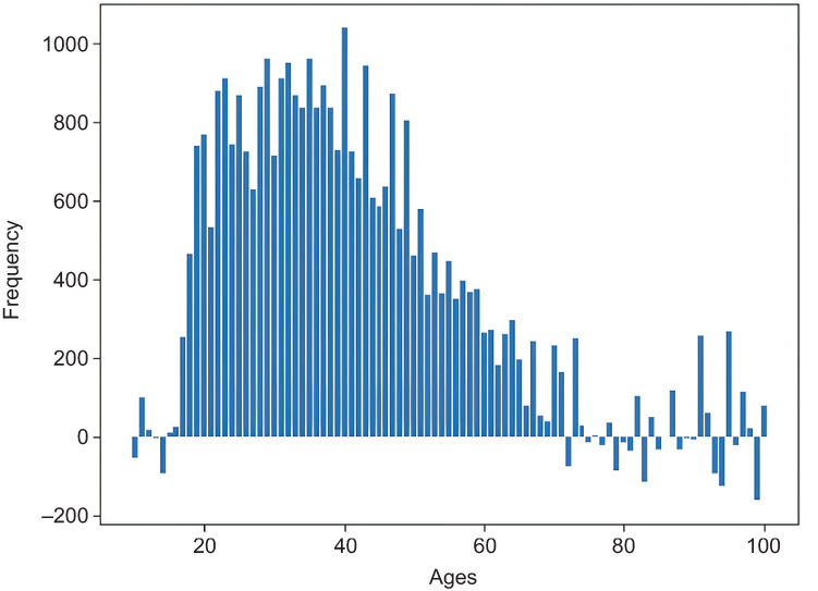
Figure 4.8 Summation of estimated ages using SHE

As you can see from figure 4.8, estimated values using SHE have a shape similar to the original encoded histogram in figure 4.7. However, the histogram in figure 4.8 is generated using an estimation function. Those estimated values have noise in them, so they are not real, and they can result in negative values. A negative age frequency is invalid for this example, so we can discard those values.

Thresholding with histogram encoding (THE)

In the case of thresholding with histogram encoding (THE), the data aggregator sets all values greater than a threshold θ to 1, and the remaining values to 0. Then it estimates the number of is in the population as E_i = (c_i - n ⋅ q)/(p - q), where p = 1 − 1/2e^{(ϵ⋅(1-θ)/2)}, q = e^{(ϵ⋅(0-θ)/2)}, and c_i is the number of 1s in the ith components of all reported values after applying thresholding.

The following listing shows the implementation of the perturbation using THE.

Listing 4.15 Thresholding with histogram encoding

def the_perturbation(encoded_ans, epsilon = 5.0, theta = 1.0):
    return [the_perturb_bit(b, epsilon, theta) for b in encoded_ans]

def the_perturb_bit(bit, epsilon = 5.0, theta = 1.0):
    val = bit + np.random.laplace(loc=0, scale = 2 / epsilon)

    if val > theta:
        return 1.0
    else:
        return 0.0

print(the_perturbation(encoding(11)))                                     ❶
print()

print(the_perturbation(encoding(11), epsilon = .1))                       ❷

the_perturbed_answers = np.sum([the_perturbation(encoding(r)) 
➥ for r in adult_age], axis=0)                                           ❸
plt.bar(domain, the_perturbed_answers)
plt.ylabel('Frequency')
plt.xlabel('Ages')

def the_aggregation_and_estimation(answers, epsilon = 5.0, theta = 1.0):  ❹
    p = 1 - 0.5 * pow(math.e, epsilon / 2 * (1.0 - theta))
    q = 0.5 * pow(math.e, epsilon / 2 * (0.0 - theta))
    
    sums = np.sum(answers, axis=0)
    n = len(answers)
    
    return [int((i - n * q) / (p-q)) for i in sums]  

❶ Test the perturbation, epsilon = 5.0.

❷ Test the perturbation, epsilon = .1.

❸ Total perturbation

❹ THE—aggregation and estimation

The output will look like the following for different epsilon values. Figure 4.9 shows the total perturbation before the THE estimation function.

[0.0, 1.0, 0.0, 0.0, 0.0, 0.0, 0.0, 0.0, 1.0, 0.0, 0.0, 0.0, 0.0, 0.0, 0.0, 0.0, 0.0, 0.0, 1.0, 0.0, 0.0, 0.0, 0.0, 0.0, 0.0, 1.0, 0.0, 0.0, 0.0, 0.0, 0.0, 0.0, 0.0, 0.0, 0.0, 0.0, 0.0, 0.0, 0.0, 0.0, 0.0, 0.0, 0.0, 0.0, 0.0, 0.0, 0.0, 0.0, 0.0, 0.0, 0.0, 0.0, 0.0, 0.0, 0.0, 0.0, 0.0, 0.0, 0.0, 0.0, 0.0, 0.0, 0.0, 0.0, 0.0, 0.0, 0.0, 0.0, 0.0, 0.0, 0.0, 0.0, 0.0, 0.0, 0.0, 0.0, 0.0, 0.0, 0.0, 0.0, 0.0, 0.0, 0.0, 0.0, 0.0, 0.0, 0.0, 0.0, 0.0, 0.0, 0.0]

[1.0, 1.0, 1.0, 0.0, 0.0, 0.0, 0.0, 0.0, 1.0, 0.0, 0.0, 0.0, 0.0, 0.0, 1.0, 1.0, 0.0, 1.0, 0.0, 1.0, 1.0, 0.0, 1.0, 1.0, 0.0, 0.0, 0.0, 1.0, 0.0, 0.0, 0.0, 1.0, 0.0, 0.0, 1.0, 1.0, 1.0, 0.0, 0.0, 1.0, 0.0, 0.0, 0.0, 1.0, 1.0, 1.0, 0.0, 0.0, 0.0, 1.0, 1.0, 0.0, 0.0, 0.0, 0.0, 0.0, 1.0, 0.0, 1.0, 1.0, 0.0, 1.0, 0.0, 1.0, 0.0, 0.0, 0.0, 1.0, 1.0, 1.0, 1.0, 0.0, 0.0, 0.0, 1.0, 0.0, 0.0, 0.0, 0.0, 0.0, 1.0, 1.0, 0.0, 1.0, 0.0, 1.0, 0.0, 0.0, 0.0, 0.0, 1.0]

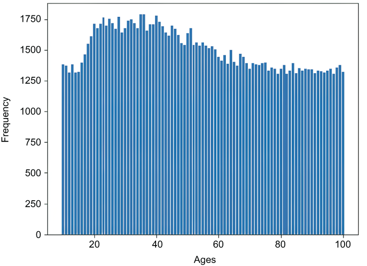
Figure 4.9 Histogram of perturbed answers using THE

The estimated values can be obtained as shown in the following code snippet:

# Data aggregation and estimation
the_perturbed_answers = [the_perturbation(encoding(r)) for r in adult_age]
estimated_answers = the_aggregation_and_estimation(the_perturbed_answers)
plt.bar(domain, estimated_answers)
plt.ylabel('Frequency')
plt.xlabel('Ages')

The output histogram is shown in figure 4.10. The estimated values of THE follow a shape similar to the original encoded histogram in figure 4.7.

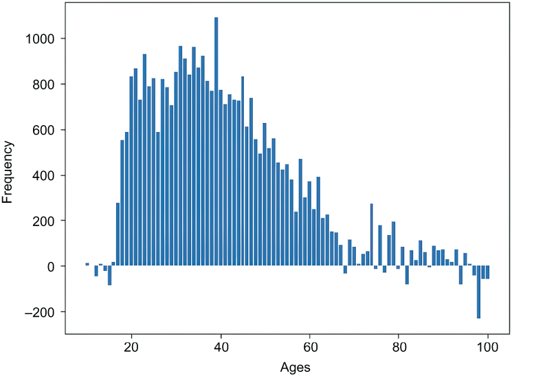
Figure 4.10 Thresholding estimated ages

In summary, histogram encoding enables us to apply LDP for numerical and continuous data, and we discussed two estimation mechanisms for LDP under histogram encoding: SHE and THE. SHE sums up the reported noisy histograms from all users, whereas THE interprets each noisy count above a threshold as 1 and each count below the threshold as 0. When you compare histogram encoding with direct encoding, you’ll realize that direct encoding has a more significant variance when the size of the domain set d becomes larger. With THE, by fixing ε, you can choose a θ value to minimize the variance. This means THE can improve the estimation over SHE because thresholding limits the effects of large amounts of noise:

• Summation with histogram encoding (SHE):

  • Encoding: Encode(v) = [0.0, 0.0,...,1.0,...,0.0] where only the vth component is 1.0.
  • Perturbation: Add Lap(2/ε) to each component.
  • Estimation: Sums up the reported noisy histograms from all individuals.

• Thresholding with histogram encoding (THE):

  • Encoding: Encode(v) = [0.0, 0.0,...,1.0,...,0.0] where only the v th component is 1.0.
  • Perturbation: Add Lap(2/ε) to each component. Set the values > θ to 1, and the remaining values to 0.
  • Estimation:  where  and .

4.2.3 Unary encoding

The unary encoding mechanism is a more general and efficient LDP mechanism for categorical and discrete problems. In this method, an individual encodes their value v as a length-d binary vector [0, ..., 1, ..., 0] where only the v th bit is 1 and the remaining bits are 0. Then, for each bit in the encoded vector, they report the value correctly with probability p and incorrectly with probability 1 - p if the input bit is 1. Otherwise, they can report correctly with probability 1 - q and incorrectly with probability q.

In unary encoding, we again have two different options to proceed with:

• Symmetric unary encoding (SUE)

• Optimal unary encoding (OUE)

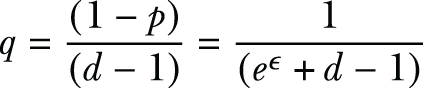
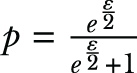
In the case of symmetric unary encoding, p is selected as  and q is selected as 1 - p. In optimal unary encoding, p is selected as 1/2 and q is selected as 1/(e^ε + 1). Then the data aggregator estimates the number of 1s in the population as E_i = (c_i - m ∙ q)/(p - q), where c_i denotes the number of 1s in the i^th bit of all reported values.

As an example of the unary encoding mechanism, suppose someone wants to determine how many people there are of different races. They would need to ask each individual the question, “What is your race?” Let’s try to implement SUE on the US Census dataset. The OUE implementation would be an extension of the SUE implementation, with changes to the definitions of p and q in the implementation. (You can also refer to the sample implementation of OUE in our code repository.)

First, let’s load the data and check the domains.

Listing 4.16 Retrieving different race categories in the dataset

import pandas as pd
import numpy as np
import matplotlib.pyplot as plt
import sys
import io
import requests
import math

req = requests.get("https://archive.ics.uci.edu/ml/machine-learning-
➥ databases/adult/adult.data").content               ❶
adult = pd.read_csv(io.StringIO(req.decode('utf-8')), 
➥ header=None, na_values='?', delimiter=r", ")
adult.dropna()
adult.head()

domain = adult[8].dropna().unique()                   ❷
domain.sort()
domain

❶ Load the data.

❷ The domains

The output of listing 4.16 will look like the following

array(['Amer-Indian-Eskimo', 'Asian-Pac-Islander', 'Black', 'Other',
       'White'], dtype=object)

As you can see, there are five different races in the dataset.

Now let’s look at the actual numbers of people of different races in the US Census dataset.

Listing 4.17 Number of people of each race

adult_race = adult[8].dropna()
adult_race.value_counts().sort_index()

Here is the output with the actual numbers in the dataset:

Amer-Indian-Eskimo      311
Asian-Pac-Islander     1039
Black                  3124
Other                   271
White                 27816

As you can see, we have 311 people in the category of “Amer-Indian-Eskimo,” 1,039 people in “Asian-Pac-Islander,” and so on.

Now let’s look into the implementation of the SUE mechanism.

Listing 4.18 Symmetric unary encoding

def encoding(answer):
    return [1 if d == answer else 0 for d in domain]

print(encoding('Amer-Indian-Eskimo'))       ❶
print(encoding('Asian-Pac-Islander'))
print(encoding('Black'))
print(encoding('Other'))
print(encoding('White'))

❶ Test the encoding.

You should get an output similar to the following:

[1, 0, 0, 0, 0]
[0, 1, 0, 0, 0]
[0, 0, 1, 0, 0]
[0, 0, 0, 1, 0]
[0, 0, 0, 0, 1]

As we discussed at the beginning of this section, the idea is that each individual encodes their value v as a length-d binary vector [0,....,1,...,0] where only the v th bit is 1 and the remaining bits are 0.

The following listing shows how you could implement the perturbation of the SUE mechanism. It is mostly self-explanatory.

Listing 4.19 Perturbation of the symmetric unary encoding

def sym_perturbation(encoded_ans, epsilon = 5.0):                        ❶
    return [sym_perturb_bit(b, epsilon) for b in encoded_ans]

def sym_perturb_bit(bit, epsilon = 5.0):
    p = pow(math.e, epsilon / 2) / (1 + pow(math.e, epsilon / 2))
    q = 1 - p

    s = np.random.random()
    if bit == 1:
        if s <= p:
            return 1
        else:
            return 0
    elif bit == 0:
        if s <= q:
            return 1
        else: 
            return 0

print(sym_perturbation(encoding('Amer-Indian-Eskimo')))                  ❷
print(sym_perturbation(encoding('Asian-Pac-Islander')))
print(sym_perturbation(encoding('Black')))
print(sym_perturbation(encoding('Other')))
print(sym_perturbation(encoding('White')))
print()

print(sym_perturbation(encoding('Amer-Indian-Eskimo'), epsilon = .1))    ❸
print(sym_perturbation(encoding('Asian-Pac-Islander'), epsilon = .1))
print(sym_perturbation(encoding('Black'), epsilon = .1))
print(sym_perturbation(encoding('Other'), epsilon = .1))
print(sym_perturbation(encoding('White'), epsilon = .1))

❶ Symmetric unary encoding—perturbation

❷ Test the perturbation, epsilon = 5.0.

❸ Test the perturbation, epsilon = .1.

The output of listing 4.19 will look like the following:

[1, 0, 0, 0, 0]
[0, 1, 0, 0, 0]
[0, 0, 1, 0, 0]
[0, 0, 0, 1, 0]
[0, 0, 0, 0, 1]

[1, 1, 0, 0, 1]
[0, 1, 1, 0, 1]
[1, 0, 1, 0, 0]
[1, 0, 0, 0, 1]
[1, 0, 0, 0, 1]

This shows two sets of vectors, similar to what we had in earlier mechanisms. The first set is with epsilon assigned 5.0, and the other is with epsilon assigned 0.1.

Now we can test it to see the perturbed answers:

sym_perturbed_answers = np.sum([sym_perturbation(encoding(r)) 
➥ for r in adult_race], axis=0)
list(zip(domain, sym_perturbed_answers))

You will have results similar to these:

[('Amer-Indian-Eskimo', 2851),
 ('Asian-Pac-Islander', 3269),
 ('Black', 5129),
 ('Other', 2590),
 ('White', 26063)]

Remember, these are only the values after the perturbation. We are not done yet!

Next comes the aggregation and estimation of the SUE mechanism.

Listing 4.20 Estimation of the symmetric unary encoding

def sym_aggregation_and_estimation(answers, epsilon = 5.0):                ❶
    p = pow(math.e, epsilon / 2) / (1 + pow(math.e, epsilon / 2))
    q = 1 - p
    
    sums = np.sum(answers, axis=0)
    n = len(answers)
    
    return [int((i - n * q) / (p-q)) for i in sums]  

sym_perturbed_answers = [sym_perturbation(encoding(r)) for r in adult_race]❷
estimated_answers = sym_aggregation_and_estimation(sym_perturbed_answers)
list(zip(domain, estimated_answers))

❶ Symmetric unary encoding—aggregation and estimation

❷ Data aggregation and estimation

The final values of the estimation will look like these:

[('Amer-Indian-Eskimo', 215),
 ('Asian-Pac-Islander', 1082),
 ('Black', 3180),
 ('Other', 196),
 ('White', 27791)] 

Now you know how SUE works. Let’s compare the actual and estimated values side by side to see what the difference looks like. If you pay close attention to table 4.3, you will understand that SUE works better with this kind of categorical data.

Table 4.3 Number of people in each race, before and after applying SUE

In this section we introduced two LDP mechanisms with unary encoding:

• Symmetric unary encoding (SUE):

  • Encoding: Encode(v) = [0, 0, ..., 1, ..., 0] where only the vth bit is 1.
  • Perturbation: Each bit is perturbed as in the binary randomized response mechanism.  for ε-LDP.
  • Estimation: For each value, use the estimation formula in the binary randomized response mechanism.

• Optimized unary encoding (OUE):

  • Encoding: Encode(v) = [0, 0, ..., 1, ..., 0] where only the vth bit is 1.
  • Perturbation: p = 1/2, q = 1/(e^ε + 1) (as shown in figure 4.11).
  • Estimation: .

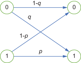
Figure 4.11 The perturbation of optimized unary encoding

This chapter mainly focused on how different LDP mechanisms work, particularly for one-dimensional data. In chapter 5, we will extend our discussion and look at how we can work with multidimensional data using more advanced mechanisms.

Summary

• Unlike centralized DP, LDP eliminates the need for a trusted data curator; thus, individuals can send their data to the data aggregator after privatizing it using perturbation techniques.

• In many practical use cases, LDP is applied for mean or frequency estimation.

• The randomized response mechanism can also be used with LDP through the design and implementation of privacy-preserving algorithms.

• While direct encoding helps us apply LDP for categorical and discreet data, histogram encoding can be used to apply LDP for numerical and continuous variables.

• When the data aggregator collects the perturbed values, the aggregator has two options for estimation methods: summation with histogram encoding (SHE) and thresholding with histogram encoding (THE).

• Summation with histogram encoding (SHE) calculates the sum of all values reported by individuals.

• In the case of thresholding with histogram encoding (THE), the data aggregator sets all values greater than a threshold θ to 1, and the remaining values to 0.

• The unary encoding mechanism is a more general and efficient LDP mechanism for categorical and discrete problems.