5 Advanced LDP mechanisms for machine learning

This chapter covers

• Advanced LDP mechanisms
• Working with naive Bayes for ML classification
• Using LDP naive Bayes for discrete features
• Using LDP naive Bayes for continuous features and multidimensional data
• Designing and analyzing an LDP ML algorithm

In the previous chapter we looked into the basic concepts and definition of local differential privacy (LDP), along with its underlying mechanisms and some examples. However, most of those mechanisms are explicitly designed for one-dimensional data and frequency estimation techniques, with direct encoding, histogram encoding, unary encoding, and so on. In this chapter we will extend our discussion further and look at how we can work with multidimensional data.

First, we’ll introduce an example machine learning (ML) use case with naive Bayes classification. Then, we’ll look at a case study implementation of LDP naive Bayes by designing and analyzing an LDP ML algorithm.

5.1 A quick recap of local differential privacy

As we discussed in the previous chapter, LDP is a way of measuring individual privacy when the data collector is not trusted. LDP aims to guarantee that when an individual provides a particular value, it should be difficult to identify the individual, thus providing privacy protection. Many LDP mechanisms also aim to estimate the distribution of the population as accurately as possible, based on an aggregation of perturbed data collected from multiple individuals.

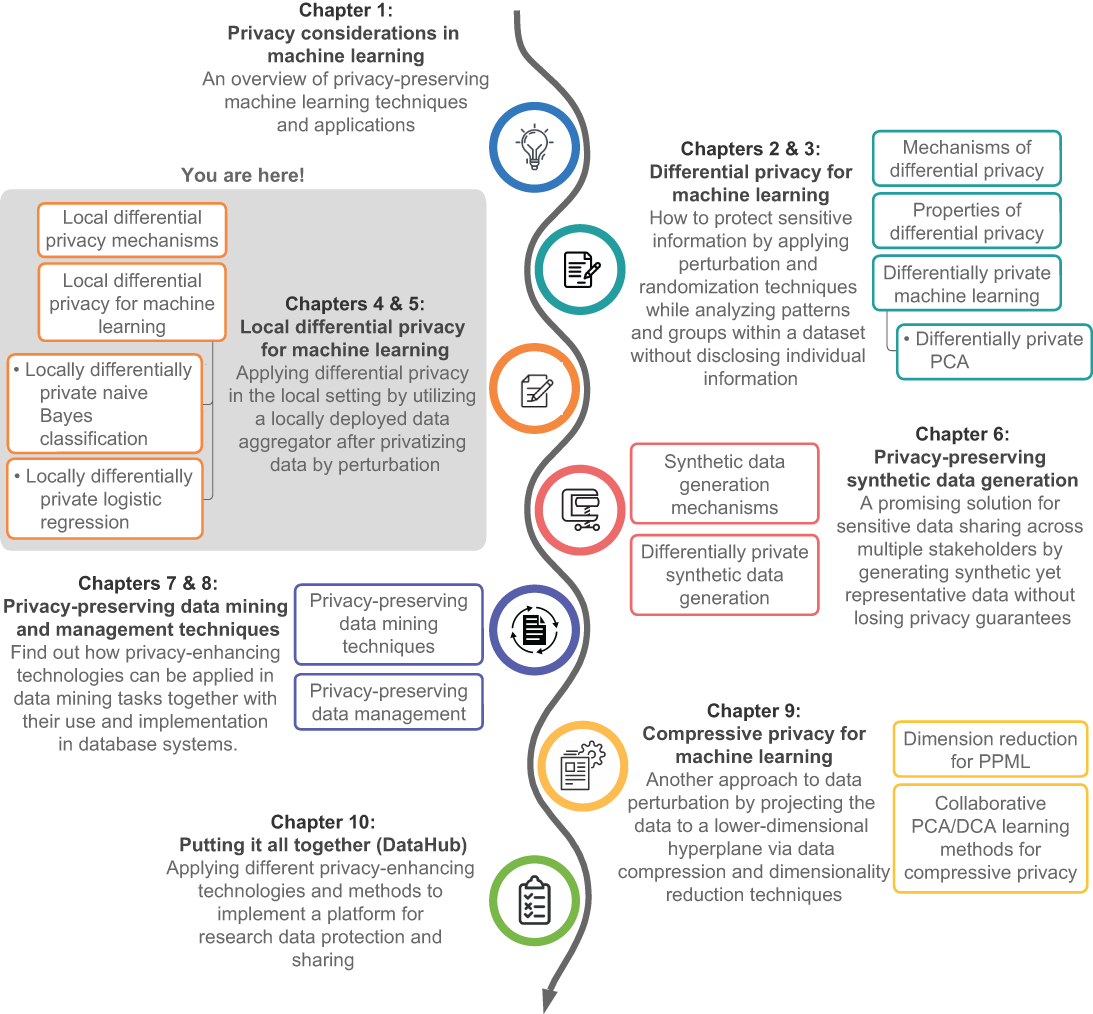
Figure 5.1 summarizes the steps of applying LDP in different application scenarios. For more about how LDP works, see chapter 4.

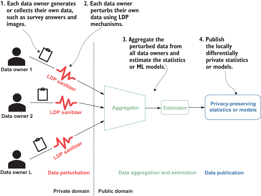
Figure 5.1 How LDP works: each data owner perturbs their data locally and submits it to the aggregator.

Now that we’ve reviewed the basics of how LDP works, let’s look at some more advanced LDP mechanisms.

5.2 Advanced LDP mechanisms

In chapter 4 we looked at the direct encoding, histogram encoding, and unary encoding LDP mechanisms. Those algorithms all work for one-dimensional categorical data or discrete numerical data. For example, the answer to the survey question “What is your occupation?” will be one occupation category, which is one-dimensional categorical data. The answer to the survey question “What is your age?” will be a one-dimensional discrete numerical value. However, many other datasets, especially when working with ML tasks, are more complex and contain multidimensional continuous numerical data. For instance, pixel-based images are usually high-dimensional, and mobile-device sensor data (such as gyroscope or accelerometer sensors) is multidimensional, usually continuous, numerical data. Therefore, learning about the LDP mechanisms that deal with such scenarios in ML tasks is essential.

In this section we’ll focus on three different mechanisms that are designed for multidimensional continuous numerical data: the Laplace mechanism, Duchi’s mechanism, and the Piecewise mechanism.

5.2.1 The Laplace mechanism for LDP

In chapter 2 we introduced the Laplace mechanism for centralized differential privacy. We can similarly implement the Laplace mechanism for LDP. First, though, let’s review some basics.

For simplicity, let’s assume each participant in the LDP mechanism is u_i and that each u_i’s data record is t_i. This t_i is a usually one-dimensional numerical value in the range of -1 to 1 (as discussed in the previous chapter), and we can mathematically represent it as t_i ∈ [-1,1]^d. However, in this section we are going to discuss multidimensional data, so t_i can be defined as a d-dimensional numerical vector in the range of -1 to 1 as t_i ∈ [-1, 1]^d. In addition, we are going to perturb t_i with the Laplace mechanism, so we’ll let t_i^* denote the perturbed data record of t_i after applying LDP.

With those basics covered, we can now dig into the Laplace mechanism for LDP. Let’s say we have a participant u_i, and their data record is t_i ∈ [-1,1]^d. Remember, this data record is now multidimensional. In order to satisfy LDP, we need to perturb this data record, and in this case we are going to use noise generated from a Laplace distribution. We’ll define a randomized function t_i^* = t_i + Lap(2 * d/ϵ) to generate a perturbed valuet_i^*, where Lap(λ) is a random variable from a Laplace distribution of scale λ.

Tip Are you wondering why we are always looking at the Laplace mechanism when it comes to differential privacy? The reason is that Gaussian perturbations are not always satisfactory, since they cannot be used to achieve pure DP (ϵ-DP), which requires heavier-tailed distributions. Thus, the most popular distribution is the Laplace mechanism, whose tails are “just right” for achieving pure DP.

The following listing shows the Python code that implements the Laplace mechanism for LDP.

Listing 5.1 The Laplace mechanism for LDP

def getNoisyAns_Lap(t_i, epsilon):
    loc = 0
    d = t_i.shape[0]
    scale = 2 * d / epsilon
    s = np.random.laplace(loc, scale, t_i.shape)
    t_star = t_i + s
    return t_star

The Laplace mechanism provides the basic functionality to perturb multidimensional continuous numerical data for LDP. However, as studied by Wang et al. [1], when using a smaller privacy budget ϵ (i.e., ϵ < 2.3), the Laplace mechanism tends to result in more variance in the perturbed data, thus providing bad utility performance. In the next section we’ll look into the Duchi’s mechanism, which performs better when using a smaller privacy budget.

5.2.2 Duchi’s mechanism for LDP

While the Laplace mechanism is one way to generate noise for the perturbation that is used with LDP, Duchi et al. [2] introduced another approach, known as Duchi’s mechanism, to perturb multidimensional continuous numerical data for LDP. The concept is similar to the Laplace mechanism, but the data perturbation is handled differently.

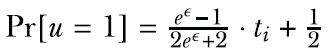
Let’s first look at how Duchi’s mechanism handles perturbation for one-dimensional numerical data. Given a participant u_i, their one-dimensional data record t_i ∈ [-1,1], and a privacy budget ϵ, Duchi’s mechanism performs as follows:

1. A Bernoulli variable u is sampled such that .

2. Then, if u = 1, the perturbed data will be ; otherwise, it is .

3. The perturbed data will be the output of Duchi’s mechanism.

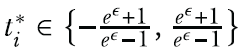
The Python implementation of this algorithm is shown in the following listing.

Listing 5.2 Duchi’s mechanism for one-dimensional data

def Duchi_1d(t_i, eps, t_star):
    p = (math.exp(eps) - 1) / (2 * math.exp(eps) + 2) * t_i + 0.5
    coin = np.random.binomial(1, p)
    if coin == 1:
        return t_star[1]
    else:
        return t_star[0]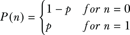

Now that you know how Duchi’s mechanism works for one-dimensional data, let’s extend it for multidimensional data. Given a d-dimensional data record t_i ∈ [-1,1]^d and the privacy budget ϵ, Duchi’s mechanism for multidimensional data performs as follows:

1. Generate a random d-dimensional data record v ∈ [-1,1]^d by sampling each v[A_j] independently from the following distribution,

   

   where v[A_j] is the jth value of v.

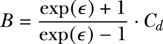
2. Define T⁺ (resp. T^-) as the set of all data records t ^* ∈ {-B, B}^d such that t^* ⋅ v ≥ 0 (resp. t^* ⋅ v ≤ 0), where we have

   

   

3. A Bernoulli variable u is sampled such that .

4. Finally, if u = 1, output a data record uniformly selected from T⁺; otherwise, output a data record uniformly selected from T^-.

The following listing shows the Python implementation of this algorithm. If you carefully follow the steps we just discussed, you will quickly understand what we are doing in the code.

Listing 5.3 Duchi’s mechanism for multidimensional data

def Duchi_md(t_i, eps):
    d = len(t_i)
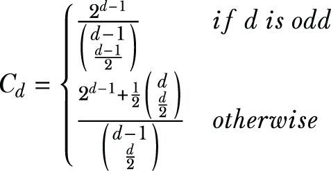
    if d % 2 != 0:
        C_d = pow(2, d - 1) / comb(d - 1, (d - 1) / 2)
    else:
        C_d = (pow(2, d - 1) + 0.5 * comb(d, d / 2)) / comb(d - 1, d / 2)
 
    B = C_d * (math.exp(eps) + 1) / (math.exp(eps) - 1)
    v = []
    for tmp in t_i:
        tmp_p = 0.5 + 0.5 * tmp
        tmp_q = 0.5 - 0.5 * tmp
        v.append(np.random.choice([1, -1], p=[tmp_p, tmp_q]))
    bernoulli_p = math.exp(eps) / (math.exp(eps) + 1)
    coin = np.random.binomial(1, bernoulli_p)
 
    t_star = np.random.choice([-B, B], len(t_i), p=[0.5, 0.5])
    v_times_t_star = np.multiply(v, t_star)
    sum_v_times_t_star = np.sum(v_times_t_star)
    if coin == 1:
        while sum_v_times_t_star <= 0:
            t_star = np.random.choice([-B, B], len(t_i), p=[0.5, 0.5])
            v_times_t_star = np.multiply(v, t_star)
            sum_v_times_t_star = np.sum(v_times_t_star)
    else:
        while sum_v_times_t_star > 0:
            t_star = np.random.choice([-B, B], len(t_i), p=[0.5, 0.5])
            v_times_t_star = np.multiply(v, t_star)
            sum_v_times_t_star = np.sum(v_times_t_star)
return t_star.reshape(-1)

Duchi’s mechanism performs well with a smaller privacy budget (i.e., ϵ < 2.3). However, it performs worse than the Laplace mechanism in terms of the utility when you are using a larger privacy budget. Could there be a more general algorithm that works well regardless of whether the privacy budget is small or large? We’ll look at the Piecewise mechanism in the next section.

5.2.3 The Piecewise mechanism for LDP

So far in this chapter you’ve learned about mechanisms that can be used for LDP. A third mechanism, called the Piecewise mechanism [1], had been proposed to deal with multidimensional continuous numerical data when using LDP, and it can overcome the disadvantages of the Laplace and Duchi’s mechanisms. The idea is to perturb multidimensional numerical values with an asymptotic optimal error bound. Hence, it requires only one bit for each individual to be reported to the data aggregator.

First, let’s look at the Piecewise mechanism for one-dimensional data. Given the participant u_i’s one-dimensional data record t_i ∈ [-1,1] and privacy budget ϵ, the Piecewise mechanism performs as follows:

1. A value x is selected in the range of 0 to 1, uniformly at random.

2. If , we sample t_i^* uniformly at random from [l(t_i), r(t_i)]; otherwise, we sample t_i^* uniformly at random from [-C, l(t_i) ∪ r(t_i), C], where

   

   

   and

   

3. Perturbed data t_i^* ∈{-C,C} will be the output of the Piecewise mechanism.

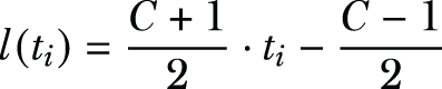
The Piecewise mechanism consists of three pieces: the center piece, the right piece r(), and the left piece l(). The centerpiece is calculated as t_i* ∈ [l(t_i), r(t_i)], the rightmost piece as t_i* ∈ [r(t_i),C], and the leftmost piece as t_i* ∈ [-C, l(t_i)]. You can see a Python implementation of this algorithm in the following listing.

Listing 5.4 Piecewise mechanism for one-dimensional data

def PM_1d(t_i, eps):
    C = (math.exp(eps / 2) + 1) / (math.exp(eps / 2) - 1)
    l_t_i = (C + 1) * t_i / 2 - (C - 1) / 2
    r_t_i = l_t_i + C - 1
    
    x = np.random.uniform(0, 1)                              ❶
    threshold = math.exp(eps / 2) / (math.exp(eps / 2) + 1)
    if x < threshold:
        t_star = np.random.uniform(l_t_i, r_t_i)
    else:
        tmp_l = np.random.uniform(-C, l_t_i)
        tmp_r = np.random.uniform(r_t_i, C)
        w = np.random.randint(2)
        t_star = (1 - w) * tmp_l + w * tmp_r
    
    return t_star

❶ Providing the size parameter in uniform() would result in an ndarray.

How can we deal with multidimensional data? We can simply extend the Piecewise mechanism from its one-dimensional version to work with multidimensional data. Given a d-dimensional data record t_i ∈ [-1,1]^d and a privacy budget ϵ, the Piecewise mechanism for multidimensional data performs as follows:

1. Sample k values uniformly without replacement from {1, 2, ..., d}, where

   

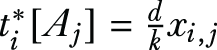
2. For each sampled value j, feed t_i[A_j] and  as the input to the one-dimensional version of the Piecewise mechanism and obtain a noisy value x_i,j.

3. Output t_i^*, where .

The following listing shows a Python implementation of this algorithm.

Listing 5.5 Piecewise mechanism for multidimensional data

def PM_md(t_i, eps):
    d = len(t_i)
    k = max(1, min(d, int(eps / 2.5)))
    rand_features = np.random.randint(0, d, size=k)
    res = np.zeros(t_i.shape)
    for j in rand_features:
        res[j] = (d * 1.0 / k) * PM_1d(t_i[j], eps / k)
    return res

Now that we have studied three advanced LDP mechanisms for multidimensional numerical data, let’s look at a case study showing how LDP can be implemented with real-world datasets.

5.3 A case study implementing LDP naive Bayes classification

In the previous chapter we introduced a set of mechanisms that can be used to implement LDP protocols. In this section we’ll use the LDP naive Bayes classification design as a case study to walk through the process of designing an LDP ML algorithm. The content in this section has been partially published in one of our research papers [3]. The implementation and the complete code for this case study can be found at https://github.com/nogrady/PPML/tree/main/Ch5.

NOTE This section will walk you through the mathematical formulations and empirical evaluations for this case study so that you can learn how to develop an LDP application from scratch. If you do not need to know these implementation details right now, you can skip ahead to the next chapter.

5.3.1 Using naive Bayes with ML classification

In section 3.2.1 you learned how differentially private naive Bayes classification works and its mathematical formulations. In this section we will broaden the discussion and explore how we can use naive Bayes with LDP. As discussed in the previous chapter, LDP involves individuals sending their data to the data aggregator after privatizing the data by perturbation. These techniques provide plausible deniability for individuals. The data aggregator then collects all the perturbed values and estimates statistics such as the frequency of each value in the population.

To guarantee the privacy of the individuals who provide training data in a classification task, LDP techniques can be used at the data collection stage. In this chapter we’ll apply LDP techniques to naive Bayes classifiers, which are a set of simple probabilistic classifiers based on Bayes’ theorem. To quickly recap, naive Bayes classifiers assume independence between every pair of features. Most importantly, these classifiers are highly scalable and particularly suitable when the number of features is high or when the training data is small. Naive Bayes can often perform better than or close to more sophisticated classification methods, despite its simplicity.

Let’s get into the details now. Given a new instance (a known class value), naive Bayes computes the conditional probability of each class label and then assigns the class label with maximum likelihood to the given instance. The idea is that, using Bayes’ theorem and the assumption of independence of features, each conditional probability can be decomposed as the multiplication of several probabilities. We need to compute each of these probabilities using training data to achieve naive Bayes classification. Since the training data must be collected from individuals by preserving privacy, we can utilize LDP frequency and statistical estimation methods to collect perturbed data from individuals and then estimate conditional probabilities with the naive Bayes classification.

In this case study, we’ll first look into how we can work with discrete features using an LDP naive Bayes classifier by preserving the relationships between the class labels and the features. Second, we’ll walk through the case of continuous features. We’ll discuss how we can discretize data and apply Gaussian naive Bayes after adding Laplace noise to the data to satisfy LDP. We will also show you how to work with continuous data perturbation methods. Finally, we’ll explore and implement these techniques with a set of experimental scenarios and real datasets, showing you how LDP guarantees are satisfied while maintaining the accuracy of the classifier.

5.3.2 Using LDP naive Bayes with discrete features

Before digging into the theory, let’s first look at an example. An independent analyst wants to train an ML classifier to predict “how likely a person is to miss a mortgage payment.” The idea is to use data from different mortgage and financial companies, train a model, and use this model to predict the behavior of future customers. The problem is that none of the financial companies want to participate because they do not want to share their customers’ private or sensitive information. The best option for them is to share a perturbed version of their data so that their customers’ privacy is preserved. But how can we perturb the data so that it can be used to train a naive Bayes classifier while protecting privacy? That’s what we are going to find out.

We discussed how naive Bayes classification works in section 3.2.1, so we’ll only recap the essential points here. Refer back to chapter 3 for more details.

In probability theory, Bayes’ theorem describes the probability of an event, based on prior knowledge of conditions that might be related to the event. It is stated as follows:

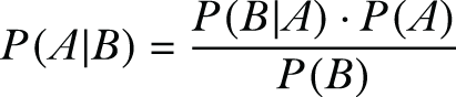
The naive Bayes classification technique uses Bayes’ theorem and the assumption of independence between every pair of features. Suppose the instance to be classified is the n-dimensional vector X = {x₁, x₂, ..., x_n}, the names of the features are F₁, F₂, ..., F_n, and the possible classes that can be assigned to the instance are C = {C₁, C₂, ..., C_k}. A naive Bayes classifier assigns the instance X to the class C_s if and only if P(C_s|X) > P(C_j|X) for 1 ≤ j ≤ k and j ≠ s. Hence, the classifier needs to compute P(C_j|X) for all classes and compare these probabilities. Using Bayes’ theorem, the probability P(C_j|X) can be calculated as

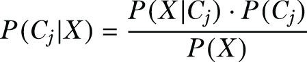
Since P(X) is same for all classes, it is sufficient to find the class with the maximum P(X|C_j) ∙ P(C_j).

Let’s first consider the case where all the features are numerical and discrete. Suppose there are m different records or individuals (among these financial companies) that can be used to train this classifier. Table 5.1 shows an extract from a mortgage payment dataset that we discussed in chapter 3.

Table 5.1 An extract from a dataset of mortgage payments. Age, income, and gender are the independent variables, whereas missed payment represents the dependent variable for the prediction task.

Our objective is to use this data to train a classifier that can be used to predict future customers and to determine whether a particular customer is likely to miss a mortgage payment or not. Thus, in this case, the classification task is the prediction of the customer’s behavior (whether they will miss a mortgage payment or not), which makes it a binary classification—we only have two possible classes.

Much as we did in chapter 3, let’s define these two classes as C₁ and C₂ where C₁ represents missing a previous payment and C₂ represents otherwise. Based on the data reported in table 5.1, the probabilities of these classes can be computed as follows:

Similarly, we can compute the conditional probabilities. Table 5.2 summarizes the conditional probabilities we already calculated in chapter 3 for the age feature.

Table 5.2 A summary of conditional probabilities computed for the age feature

Once we have all the conditional probabilities, we can predict whether, for example, a young female with medium income will miss a payment or not. To do that, first we need to set X as X = (Age = Young, Income = Medium, Gender = Female). Chapter 3 presents the remaining steps and computations for using the naive Bayes classifier, and you can refer back if necessary.

Based on the results of these computations, the naive Bayes classifier will assign C₂ for the instance X. In other words, a young female with medium income will not miss a payment.

and

With this basic understanding of how the naive Bayes classifier works, let’s see how we can use the LDP frequency estimation methods discussed earlier to compute the necessary probabilities for a naive Bayes classifier. Remember, in LDP, the data aggregator is the one that computes the class probabilities P(C_j) for all classes in C = {C₁, C₂, ..., C_k} and conditional probabilities P(F_i = x_i|C_j) for all possible x_i values.

Suppose an individual’s data, Alice’s data, is (a₁, a₂, ..., a_n) and her class label is C_v. In order to satisfy LDP, she needs to prepare her input and perturb it. Let’s look at the details of how Alice’s data can be prepared and perturbed and how the class probabilities and the conditional probabilities can be estimated by the data aggregator.

Computing class probabilities

For the computation of class probabilities, Alice’s input becomes v ∈ {1, 2, ..., k} since her class label is C_v. Then Alice encodes and perturbs her value v and reports to the data aggregator. Any LDP frequency estimation method we discussed earlier can be used. Similarly, other individuals report their perturbed class labels to the data aggregator.

The data aggregator collects all the perturbed data and estimates the frequency of each value j ∈ {1, 2, ..., k} as E_j. Now the probability P(C_j) is estimated as

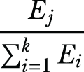
Let’s consider an example to make it clearer. There are only two options for the class label in the example dataset in table 5.1: missing a payment or not. Let’s say Alice has a missing payment. Then Alice’s input v becomes 1 and she reports it to the data aggregator. Similarly, if she does not have a missing payment, she would report 2 as her input to the data aggregator. Figure 5.2 shows three people submitting their perturbed values to the data aggregator. The data aggregator then estimates the frequency of each value and calculates the class probabilities.

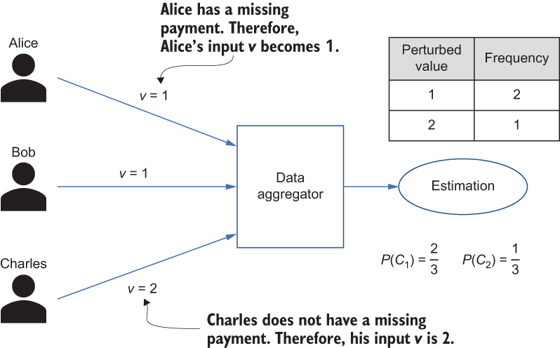
Figure 5.2 An example showing how to compute class probabilities

Computing conditional probabilities

In order to estimate the conditional probabilities P(F_i = x_i|C_j), it is not sufficient to report the feature values directly. To compute these probabilities, the relationship between class labels and features must be preserved, which means individuals need to prepare their inputs using a combination of feature values and class labels.

We’ll let the total number of possible values for F_i be n_i. If Alice’s value in ith dimension is a_i ∈ {1, 2, ..., n_i} and her class label value is v ∈ {1, 2, ..., k}, then Alice’s input for feature F_i becomes v_i = (a_i - 1)∙k + v. Therefore, each individual calculates her input for the ith feature in the range of [1, k∙n_i].

It’s a bit hard to follow, isn’t it? But don’t worry. Let’s look at this through an example. For instance, suppose the age values in table 5.1 are enumerated as (Young = 1), (Medium = 2), (Old = 3). For this age feature, an individual’s input can be a value from 1 to 6, as shown in table 5.3, where 1 represents that the age is young and there is a missing payment, and 6 represents that the age is old and there is no missing payment.

Table 5.3 Preparing input as a combination of feature values and class labels

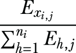
You may have noticed that there is one input value for each line in table 5.2. Similarly, the number of possible inputs for income is 6, and the number of possible inputs for gender is 4. After determining her input in the ith feature, Alice encodes and perturbs her value v_i, and reports the perturbed value to the data aggregator. To estimate the conditional probabilities for F_i , the data aggregator estimates the frequency of individuals having the value y ∈ {1, 2, ..., n_i} and class label z ∈ {1, 2, ..., k} as E_y,z by estimating the frequency of input (y - 1)∙ k + z. Hence, the conditional probability P(F_i = x_i|C_j) is estimated as

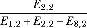
For the example in table 5.3, to estimate the probability P(Age = Medium|C₂), the data aggregator estimates the frequency of 2, 4, and 6 as E_1,2, E_2,2, and E_3,2, respectively. Then P(Age = Medium|C₂) can be estimated as

It is noteworthy that in order to contribute to the computation of class probabilities and conditional probabilities, each individual can prepare n + 1 inputs (i.e., {v, v₁, v₂, ...., v_n} for Alice) that can be reported after perturbation. However, reporting multiple values that are dependent on each other usually decreases the privacy level. Hence, each individual reports only one input value.

Finally, when the data aggregator estimates a value such as E_j or E_(y,z), the estimate may be negative. We can set all negative estimates to 1 to obtain a valid and reasonable probability.

Using LDP with multidimensional data

The aforementioned frequency and mean estimation methods only work for one-dimensional data. But what if we have higher-dimensional data? If the data owned by individuals is multidimensional, reporting each value with these methods may cause privacy leaks due to the dependence on features.

To that end, three common approaches can be used with n-dimensional data:

• Approach 1—The Laplace mechanism (discussed in chapter 3) could be used with LDP if the noise is scaled with the number of dimensions n. Hence, if an individual’s input is V = (v₁, ..., v_n) such that v_i ∈ [-1,1] for all i ∈ {1, ..., n}, individuals can report each v_i after adding Lap(2n/ε). However, this approach is not suitable if the number of dimensions n is high, because a large amount of noise reduces the accuracy.

• Approach 2—We could utilize the Piecewise mechanism that we described in section 5.2.3. The Piecewise mechanism can be used to perturb multidimensional numerical values with LDP protocols.

• Approach 3—The data aggregator can request only one perturbed input from each individual to satisfy ϵ-LDP. Each individual can select the input to be reported uniformly at random, or the data aggregator can divide the individuals into n groups and request different input values from each group. As a result, each feature is approximately reported by m/n individuals. This approach is suitable when the number of individuals m is high, relative to the number of features n. Otherwise, the accuracy decreases, since the number of reported values is low for each feature.

Now that we’ve looked at how multidimensional data works with LDP, let’s look at the details of LDP in naive Bayes classification for continuous data.

5.3.3 Using LDP naive Bayes with continuous features

So far, we’ve seen how to apply LDP for discrete features. Now we’re going to explore how we can use the same concept for continuous features. LDP in naive Bayes classification for continuous data can be approached in two different ways:

• We can discretize the continuous data and apply the discrete naive Bayes solution outlined in the previous section. In that case, continuous numerical data is divided into buckets to make it finite and discrete. Each individual perturbs their input after discretization.

• The data aggregator can use Gaussian naive Bayes to estimate the probabilities.

Let’s start with the first approach, discrete naive Bayes.

Discrete naive Bayes

For discrete naive Bayes, we need to discretize the continuous data and use LDP frequency estimation techniques to estimate the frequency. Based on known features within a continuous domain, the data aggregator determines the intervals for the buckets in order to discretize the domain—Equal-Width Discretization (EWD) or Equal-Width Binning (EWB) can be used to equally partition the domain. EWD computes the width of each bin as (max - min)/n_b where max and min are the maximum and minimum feature values and n_b is the number of desired bins. In section 5.3.4, we’ll use the EWD method in some experiments for discretization.

When the data aggregator shares the intervals with individuals, each individual discretizes their continuous feature values and applies a procedure similar to what we discussed for LDP naive Bayes with discrete features. The data aggregator also estimates the probabilities using the same procedure as for LDP naive Bayes for discrete data. Each individual should report just one perturbed value to guarantee ϵ-LDP. As you can see, discretization through binning is a kind of data preprocessing approach. The actual privacy protection is achieved through discrete naive Bayes.

Gaussian naive Bayes

The second approach for continuous data is using Gaussian naive Bayes. In this case, the most common practice is to assume the data is normally distributed. For LDP Gaussian naive Bayes, computing class probabilities is the same as for discrete features. To compute conditional probabilities, the data aggregator needs to have the mean and the variance of the training values for each feature given a class label. In other words, to compute P(F_i = x_i|C_j), the data aggregator needs to estimate the mean μ_(i,j) and the variance σ²_i,j using the F_i values of individuals with class label C_j. That means the association between features and class labels has to be maintained (similar to the discrete naive Bayes classifier).

We already discussed the mean estimation process, but to compute the mean μ_(i,j) and the variance σ²_i,j together, the data aggregator can divide the individuals into two groups. One group contributes to the estimation of the mean (i.e., μ_(i,j)) by perturbing their inputs and sharing them with the data aggregator. The other group contributes to estimating the mean of squares (i.e., μ^S_i,j) by perturbing the squares of their inputs and sharing them with the data aggregator.

Let’s consider another example. Suppose Bob has class label C_j and a feature F_i with a value b_i. Let’s also assume that the domain of each feature is normalized to have a value between [-1,1]. If Bob is in the first group, he would add the Laplace noise to his value b_i and obtain the perturbed feature value b'_i. When the data aggregator collects all perturbed feature values from individuals in the first group having class label C_j, it computes the mean of the perturbed feature values, which gives an estimate of the mean μ_(i,j) because the mean of the noise added by individuals is 0. A similar approach could be followed by the second group. If Bob is in the second group, he would add noise to his squared value b²_i to obtain b^2'_i and would share it with the data aggregator. Again, the data aggregator computes the estimate of the mean of squares (μ^S_i,j). Finally, the variance σ²_i,j can be computed as μ^S_i,j - (μ_i,j)². Once again, each individual reports only one of their values or squares of their values after perturbation because they are dependent.

Thus far, the calculation of probabilities is clear and straightforward. But did you notice that when we calculate the mean and the variance, the class labels of individuals are not hidden from the data aggregator? How can we hide the original class labels?

To overcome this problem and hide the class labels, we can adopt the following approach: let’s say Bob is reporting a feature value F_i = b_i associated with class C_j where j ∈ {1,2, ..., k}. First he constructs a vector of length k where k is the number of class labels. The vector is initialized to zeros except for the jth element corresponding to the jth class label, which is set to the feature value b_i. After that, each element of the vector is perturbed as usual (i.e., by adding the Laplace noise) and contributed to the data aggregator. Since noise is added even to the zero elements of the vector, the data aggregator will not be able to deduce the actual class label, or the actual values.

As for estimating the actual mean value (and the mean of the squared values) for each class, the data aggregator only needs to compute the mean of the perturbed values as usual and then divide by the probability of that class. To understand why we need to do that, assume that a class j has probability P(C_j). Thus, for a feature F_i, only P(C_j) of the individuals have their actual values in the jth element of the input vector, while the remaining proportion (1 - P(C_j)) have zeros. Hence, after the noise clustered around the actual mean cancels each other, and the noise clustered around zero cancels each other, we will have P(C_j) × μ_(i,j) = observed (shifted) mean. Thereafter, we can divide the observed mean by P(C_j) to obtain the estimated mean. The same applies to the mean of the squared values and hence for computing the variance.

5.3.4 Evaluating the performance of different LDP protocols

Now that we have gone through the theory, it’s time to discuss the implementation strategies and the results of the experimental evaluation of different LDP protocols. These experiments are based on datasets obtained from the UCI Machine Learning Repository [4]. Table 5.4 summarizes the datasets used in the experiments.

Table 5.4 A summary of datasets used in the experiments

To evaluate the accuracy of naive Bayes classification under LDP, we implemented the methods discussed in the previous sections in Python utilizing the pandas and NumPy libraries. We implemented five different LDP protocols for frequency estimation—direct encoding (DE), summation with histogram encoding (SHE), thresholding with histogram encoding (THE), symmetric unary encoding (SUE), and optimal unary encoding (OUE)—and the experiments were performed with different θ values in THE. With these experiments, we found that the best accuracy can be achieved whenever θ = 0.25, so we’ll give the experimental results of SHE for θ = 0.25. In a nutshell, we will compare the results of these different implementations to show you which algorithm works best for each of these datasets.

Evaluating LDP naive Bayes with discrete features

To evaluate the accuracy of using LDP naive Bayes for classifying data with discrete features, four different datasets from the UCI ML repository (Car evaluation, Chess, Mushroom, and Connect-4) were used. Initially, naive Bayes classification without LDP was performed as the baseline for comparing the accuracy of different encoding mechanisms under LDP.

Let’s look at the experimental results for varying ϵ values up to 5, as shown in figure 5.3. The dotted lines show accuracy without privacy. As expected, when the number of instances in the training set increases, the accuracy is better for smaller ϵ values. For instance, in the Connect-4 dataset, all protocols except SHE provide more than 65% accuracy even for very small ϵ values. Since the accuracy without privacy is approximately 75%, the accuracy of all of these protocols for ϵ values smaller than 1 is noticeable. The results are also similar for the Mushroom dataset. When it comes to ϵ = 0.5, all protocols except SHE provide nearly 90% classification accuracy.

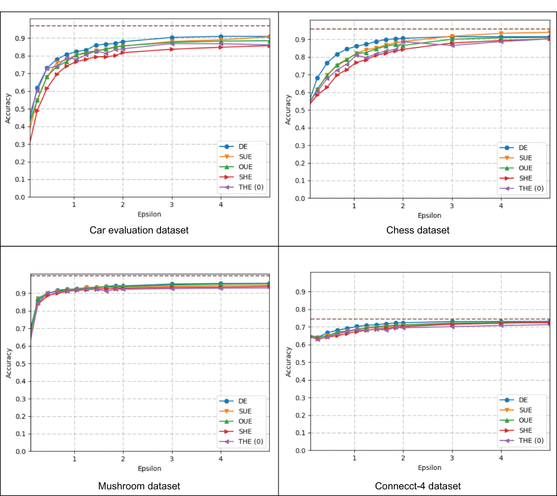
Figure 5.3 LDP naive Bayes classification accuracy for datasets with discrete features

In all of the datasets, you can see that the protocol with the worst accuracy is SHE. Since this protocol simply sums the noisy values, its variance is higher than the other protocols. In addition, DE achieves the best accuracy for small ϵ values in the Car Evaluation and Chess datasets because the input domains are small. On the other hand, the variance of DE is proportional to the size of the input domain. Therefore, its accuracy is better when the input domain is small. We can also see that SUE and OUE provide similar accuracy in all of the experiments. They perform better than DE when the size of the input domain is large. Although OUE is proposed to decrease the variance, a considerable utility difference between SUE and OUE was not observed in this set of experiments.

Evaluating LDP naive Bayes with continuous features

Now let’s discuss the results of LDP naive Bayes with continuous data. In this case, the experiments were conducted on two different datasets: Australian credit approval and Diabetes. The Australian dataset has 14 original features, and the Diabetes dataset has 8 features.

Initially, the discretization method was applied, and then two dimensionality reduction techniques (PCA and DCA) were implemented to observe their effect on accuracy. The results for the two datasets for different values of ϵ are given in figure 5.4. We also present the results for two LDP schemes, direct encoding and optimized unary encoding, which provide the best accuracy for different domain sizes. The input domain is divided into d = 2 buckets for the Australian dataset and d = 4 buckets for the Diabetes dataset.

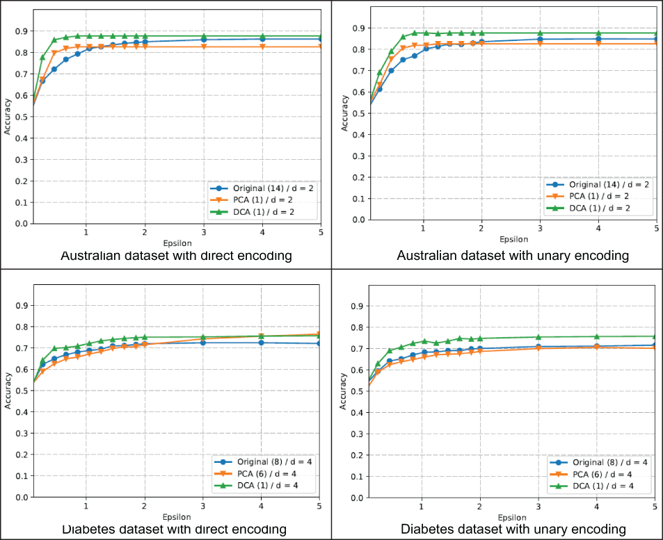
Figure 5.4 LDP naive Bayes classification accuracy for datasets with continuous features using discretization

As you can see, for the Australian dataset, the best results for principal component analysis (PCA) and discriminant component analysis (DCA) are obtained when the number of features is reduced to 1. On the other hand, for the Diabetes dataset, the best accuracy is achieved when PCA reduces the number of features to 6 and when DCA reduces the number of features to 1. As is evident in figure 5.4, DCA provides the best classification accuracy, which shows the advantage of using dimensionality reduction before discretization. You can also see that DCA’s accuracy is better than PCA’s, since DCA is mainly designed for classification.

In addition, we applied LDP Gaussian naive Bayes (LDP-GNB) on the same two datasets. All three perturbation approaches that we discussed for multidimensional data (in the subsection titled “Using LDP with multidimensional data”) were implemented. Figure 5.5 shows the results of performing LDP-GNB on these two datasets.

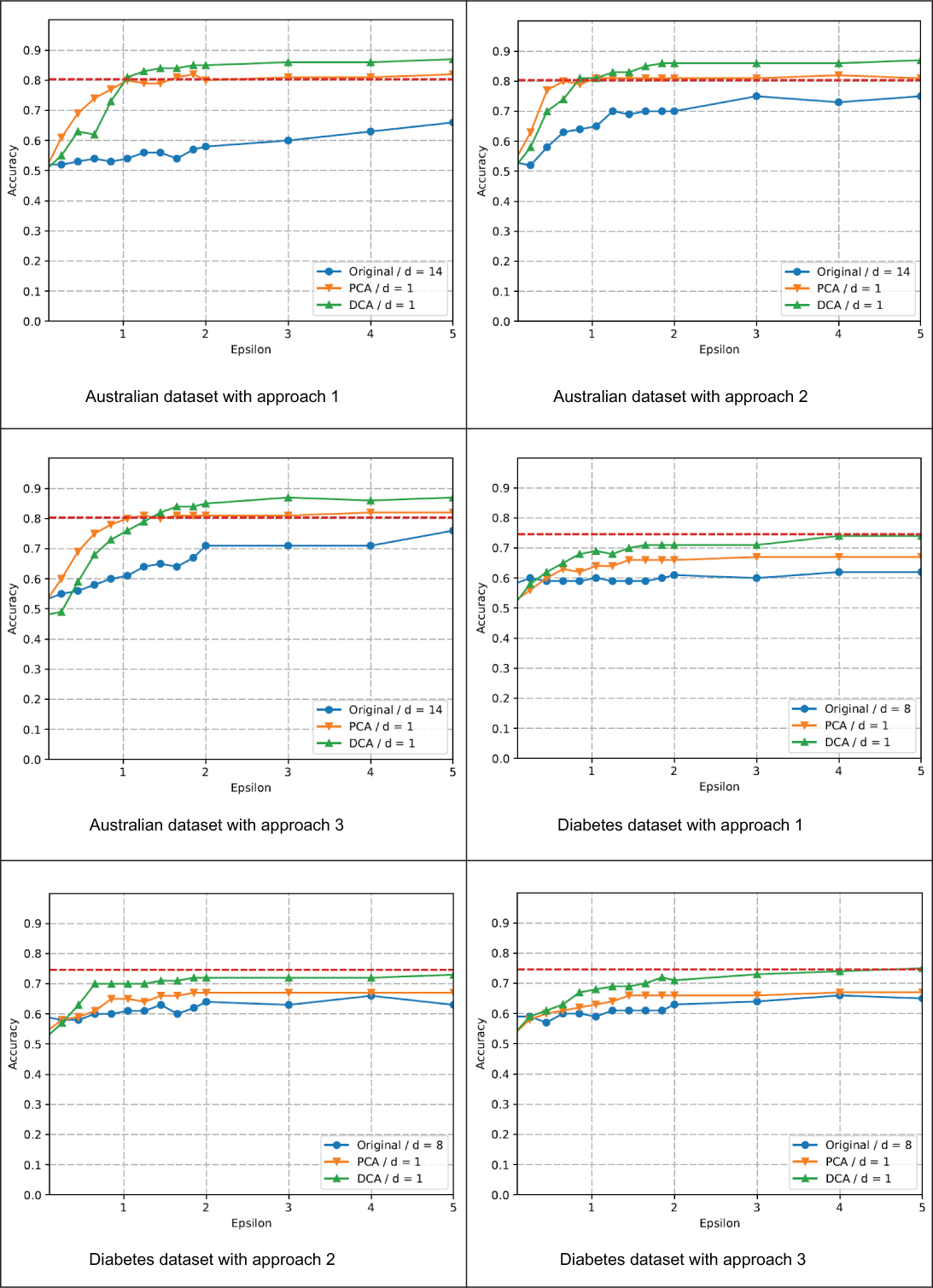
Figure 5.5 LDP Gaussian naive Bayes classification accuracy for datasets with continuous features

As you can see, the first of the three approaches (using the Laplace mechanism) results in the lowest utility, since individuals report all the features by adding more noise, proportional to the number of dimensions. In each figure, three curves are shown, corresponding to using the original data (with 14 or 8 features for the Australian and Diabetes datasets, respectively) or projecting the data using PCA or DCA before applying the LDP noise. All the graphs show the positive effect of reducing the dimensions. In both datasets, and for PCA and DCA, the number of reduced dimensions was 1. DCA or PCA always performs better than the original data and for all perturbation approaches.

Finally, when you compare the results of discretization and Gaussian naive Bayes for continuous data, you’ll see that discretization provides better accuracy. Especially for smaller ϵ values, the superiority of discretization is apparent. Although it is impossible to compare the amount of noise for randomized response and the Laplace mechanism, discretization possibly causes less noise due to the smaller input domain.

Summary

• There are different advanced LDP mechanisms that work for both one-dimensional and multidimensional data.

• As we did with the centralized setting of DP, we can implement the Laplace mechanism for LDP as well.

• While the Laplace mechanism is one way to generate noise for the perturbation, Duchi’s mechanism can also be used to perturb multidimensional continuous numerical data for LDP.

• The Piecewise mechanism can be used to deal with multidimensional continuous numerical data for LDP while overcoming the disadvantages of the Laplace and Duchi’s mechanisms.

• Naive Bayes is a simple yet powerful ML classifier that can be used with LDP frequency estimation techniques.

• LDP naive Bayes can be used with both discrete and continuous features.

• When it comes to LDP naive Bayes with continuous features, there are two main approaches, namely, discrete naive Bayes and Gaussian naive Bayes.