C H A P T E R 12
![]()
Partitioning: Divide and Conquer
If you work with large tables and indexes, at some point you'll experience performance degradation as the row counts grow into the hundreds of millions. Even efficiently written SQL statements executing against appropriately indexed tables eventually slow down as table and index sizes grow into the gigabytes, terabytes, or even higher. For such situations, you have to devise a strategy that allows your database to scale with increasing data volumes.
Oracle provides two key scalability features—parallelism and partitioning—that enable good performance even with massively large databases. Parallelism allows Oracle to start more than one thread of execution to take advantage of multiple hardware resources. Partitioning allows subsets of a table or index to be managed independently (Oracle's “divide and conquer” approach). The focus of this chapter is partitioning strategies.
Partitioning lets you create a logical table or index that consists of separate segments that can each be accessed and worked on by separate threads of execution. Each partition of a table or index has the same logical structure, such as the column definitions, but can reside in separate containers. In other words, you can store each partition in its own tablespace and associated datafiles. This allows you to manage one large logical object as a group of smaller, more maintainable pieces.
This chapter uses various terms related to partitioning. Table 12–1 describes the meanings of terms you should be familiar with.
Table 12–1. Oracle Partitioning Terminology
If you work with mainly small online transaction processing (OLTP) databases, you probably don't need to create partitioned tables and indexes. However, if you work with large OLTP databases or in data-warehouse environments, you can most likely benefit from partitioning. Partitioning is a key to designing and building scalable and highly available database systems.
What Tables Should Be Partitioned?
Following are some rules of thumb for determining whether to partition a table. In general, you should consider partitioning for
- Tables that are over 2GB in size.
- Tables that have more than 10 million rows, when SQL operations are getting slower as more data is added.
- Tables you know will grow large. It's better to create a table as partitioned rather than rebuild it as partitioned after performance begins to suffer as the table grows.
- Tables that have rows that can be divided in a way that facilitates parallel operations like loading, retrieval, or backup and recovery.
- Tables for which you want to archive the oldest partition on a periodic basis, and tables from which you want to drop the oldest partition regularly as data becomes stale.
One rule is that any table over 2GB in size is a potential candidate for partitioning. Run this query to show the top space-consuming objects in your database:
select * from (

select

 owner

,segment_name

,segment_type

,partition_name

,sum(extents) num_ext
,sum(bytes)/1024/1024 meg_tot

from dba_segments

group by owner, segment_name, segment_type, partition_name

order by sum(extents) desc)

where rownum <= 10;
Here's a snippet of the output from the query:
OWNER   SEGMENT_NAME         SEGMENT_TYPE     PARTITION_NAME  NUM_EXT  MEG_TOT

------- -------------------- ---------------- -------------- -------- --------

REP_MV  REG_QUEUE_REP_ARCH   TABLE                             29,218   29,218

REP_MV  REG_QUEUE_REP        TABLE                             15,257   15,257

STAR2   F_INSTALLATIONS      TABLE PARTITION  INST_P_6          4,092    4,092
This output shows that a few large tables in this database may benefit from partitioning. For this database, if there are performance issues with these large objects, then partitioning may help.
If you're running the previous query from SQL*Plus, you need to apply some formatting to the columns to reasonably display the output within the limited width of your terminal:
set lines 132

col owner form a10

col segment_name form a20

col partition_name form a15
In addition to looking at the size of objects, if you can divide your data so that it facilitates operations such as loading data, querying, backups, archiving, and deleting, you should consider using partitioning. For example, if you work with a large table that contains data that is often accessed by a particular time range—such as by day, week, month, or year—it makes sense to consider partitioning.
A large table size combined with a good business reason means you should consider partitioning. Keep in mind that there is more setup work and maintenance when you partition a table. However, as mentioned earlier, it's much easier to partition a table during setup than it is to convert it after it's grown to an unwieldy size.
![]() Note Partitioning is an extra-cost option that is available only with the Oracle Enterprise Edition. You have to decide based on your business requirements whether partitioning is worth the cost.
Note Partitioning is an extra-cost option that is available only with the Oracle Enterprise Edition. You have to decide based on your business requirements whether partitioning is worth the cost.
Creating Partitioned Tables
Oracle provides a robust set of methods for dividing tables and indexes into smaller subsets. For example, you can divide a table's data by date ranges, such as by month or year. Table 12–2 gives an overview of the partitioning strategies available.
Table 12–2. Partitioning Strategies
| Partition Type | Description |
| Range | Allows partitioning based on ranges of dates, numbers, or characters. |
| List | Useful when the partitions fit nicely into a list of values, like state or region codes. |
| Hash | Allows even distribution of rows when there is no obvious partitioning key. |
| Composite | Allows combinations of other partitioning strategies. |
| Interval | Extends range partitioning by automatically allocating new partitions when new partition key values exceed the existing high range. |
| Reference | Useful for partitioning a child table based on a parent table column. |
| Virtual | Allows partitioning on a virtual column. |
| System | Allows the application inserting the data to determine which partition should be used. |
The following subsections show examples of each partitioning strategy. In addition, you learn how to place partitions into separate tablespaces; to take advantage of all the benefits of partitioning, you need to understand how to assign a partition to its own tablespace.
Partitioning by Range
Range partitioning is frequently used. This strategy instructs Oracle to place rows in partitions based on ranges of values such as dates or numbers. As data is inserted into a range-partitioned table, Oracle determines which partition to place a row in based on the lower and upper bound of each range partition.
The range-based partition key is defined by the PARTITION BY RANGE clause in the CREATE TABLE statement. This determines which column is used to determine which partition a row belongs in. You'll see some examples shortly.
Each range partition requires a VALUES LESS THAN clause that identifies the non-inclusive value of the upper bound of the range. The first partition defined for a range has no lower bound. Any value less than the first partition's VALUES LESS THAN clause are inserted into the first partition. For partitions other than the first partition, the lower bound of a range is determined by the upper bound of the previous partition.
Optionally, you can create a range-partitioned table's highest partition with the MAXVALUE clause. Any row inserted that doesn't have a partition key that falls in any lower ranges is inserted into this topmost MAXVALUE partition.
Using a NUMBER for the Partition Key Column
Let's look at an example to illustrate the previous concepts. Suppose you're working in a data-warehouse environment where you typically have a fact table that stores information about an event (such as registrations, sales, downloads, and so forth). In this scenario the fact table contains a number column that represents a date. For example, the value 20110101 represents January 1, 2011. You want to partition the fact table based on this number column. This SQL statement creates a table with three partitions based on a range of numbers:
create table f_regs

(reg_count number

,d_date_id number

)

partition by range (d_date_id)(

partition p_2010 values less than (20110101),

partition p_2011 values less than (20120101),

partition p_max  values less than (maxvalue)

);
When creating a range-partitioned table, you don't have to specify a MAXVALUE partition. However, if you don't specify a partition with the MAXVALUE clause, and you attempt to insert a row that doesn't fall in any other defined ranges, you receive an error such as
ORA-14400: inserted partition key does not map to any partition
When you see that error, you have to add a partition that accommodates the partition-key value being inserted or add a partition with the MAXVALUE clause.
![]() Tip If you're using Oracle Database 11g or higher, consider using an interval partitioning strategy in which partitions are automatically added by Oracle when the high range value is exceeded. This topic is covered a bit later in the section “Creating Partitions on Demand.”
Tip If you're using Oracle Database 11g or higher, consider using an interval partitioning strategy in which partitions are automatically added by Oracle when the high range value is exceeded. This topic is covered a bit later in the section “Creating Partitions on Demand.”
You can view information about the partitioned table you just created by running the following query:
select

 table_name

,partitioning_type

,def_tablespace_name

from user_part_tables

where table_name='F_REGS';
Here's a snippet of the output:
TABLE_NAME           PARTITION DEF_TABLESPACE_NAME

-------------------- --------- -------------------------

F_REGS               RANGE     USERS
To view information about the partitions in the table, issue a query like this:
select

 table_name

,partition_name

,high_value

from user_tab_partitions

where table_name = 'F_REGS'

order by

 table_name

,partition_name;
Here's some sample output:
TABLE_NAME      PARTITION_NAME  HIGH_VALUE

--------------- --------------- ------------------------------

F_REGS          P_2010          20110101

F_REGS          P_2011          20120101

F_REGS          P_MAX           MAXVALUE
In this example, the D_DATE_ID column is the partitioning-key column. The VALUES LESS THAN clauses create the partition boundaries, which define the partition into which a row is inserted. The MAXVALUE parameter creates a partition in which to store rows that don't fit into the other defined partitions (including NULL values).
DETECTING WHEN ADDITIONAL HIGH RANGE IS REQUIRED
Using a TIMESTAMP for the Partition Key Column
You may have noticed that the example in the previous section created the column D_DATE_ID as a NUMBER data type instead of a DATE data type for the F_REGS table. One technique sometimes employed in data-warehouse environments uses an intelligent surrogate key for the primary key of the D_DATES dimension. It's intelligent because the key number represents a date. This lets you partition the fact table (F_REGS) on a range of numbers that always represent a date. Sometimes data-warehouse architects find this type of partitioning easier to work with than DATE- or TIMESTAMP-based fields.
To illustrate the previous point, the following example creates the F_REGS table with a TIMESTAMP data type for the D_DATE_DTT column:
create table f_regs

(reg_count  number

,d_date_dtt timestamp

)

partition by range (d_date_dtt)(

 partition p_2010 values less than (to_date('01-jan-2011','dd-mon-yyyy')),

 partition p_2011 values less than (to_date('01-jan-2012','dd-mon-yyyy')),

 partition p_max  values less than (maxvalue)

);
As shown in this code, I recommend that you use the TO_DATE function with a format mask to be sure there is no ambiguity about how the date should be interpreted. This technique is every bit as valid as using a NUMBER field for the partition key. Just keep in mind that whoever designs the data-warehouse tables may have a strong opinion about which technique to use.
One slight variation on this example leaves out the TO_DATE function. You must then ensure that the date string you use matches a date format recognized by Oracle. For example:
create table f_regs

(reg_count  number

,d_date_dtt timestamp

)

partition by range (d_date_dtt)(

 partition p_2010 values less than ('01-jan-11'),

 partition p_2011 values less than ('01-jan-12'),

 partition p_max  values less than (maxvalue)

);
If Oracle can't interpret a date correctly, an error is thrown:
ORA-01858: a non-numeric character was found where a numeric was expected
I recommend that you always use TO_DATE to explicitly instruct Oracle how to interpret the date. Doing so also provides a minimal level of documentation for anybody supporting the database.
Placing Partitions into Tablespaces
When you're working with large partitioned tables, I recommend that you place each partition in its own tablespace. Doing so allows you to manage the storage of each partition separate from the other partitions. This also lets you back up and recover the table partitions separately, because each partition is located in its own tablespace.
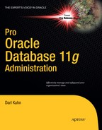
To understand the benefits of using a separate tablespace for each partition, first consider a nonpartitioned table scenario. This example creates a table and places the table into the P1_TBSP tablespace:
create table f_sales(

 sales_id  number

,amt       number

,d_date_id number)

tablespace p1_tbsp;
Now, as data is inserted into the F_SALES table, all the data is stored in the datafiles associated with the tablespace P1_TBSP. Figure 12–1 illustrates this point. There is no way for the data being inserted into a nonpartitioned table to be spread out across many tablespaces.
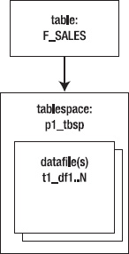
Figure 12–1. A nonpartitioned table
Compare the previous nonpartitioned architecture to that of a partitioned table. This example creates a partitioned table but doesn't specify tablespaces for the partitions:
create table f_sales (

 sales_id  number

,amt       number

,d_date_id number)
tablespace p1_tbsp

partition by range(d_date_id)(

 partition y11 values less than (20120101)

,partition y12 values less than (20130101)

,partition y13 values less than (20140101)

);
Figure 12–2 illustrates this approach. Notice that in this case, all partitions are stored in the same tablespace.
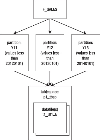
Figure 12–2. A partitioned table with only one tablespace
This approach has some advantages (over a nonpartitioned table) in that you can perform partition-maintenance operations (drop, split, merge, truncate, and so on) on one partition without affecting others (thus ensuring partition independence). However, this approach doesn't quite take advantage of all that partitioning has to offer.
The next example places each partition in a separate tablespace:
create table f_sales (

 sales_id  number

,amt       number

,d_date_id number)

tablespace p1_tbsp

partition by range(d_date_id)(

 partition y11 values less than (20120101)
   tablespace p1_tbsp

,partition y12 values less than (20130101)

    tablespace p2_tbsp

,partition y13 values less than (20140101)

    tablespace p3_tbsp

);
Now the data for each partition is physically stored in its own tablespace and corresponding datafiles (see Figure 12–3).
Figure 12–3. Partitions stored in separate tablespaces
An advantage of placing partitions in separate tablespaces is that you can back up and recover partitions independently (by backing up individual tablespaces). Also, if you have a partition that isn't being modified, you can change its tablespace to read-only and instruct utilities like Oracle Recovery Manager (RMAN) to skip backing up such tablespaces, thus increasing backup performance. Additionally, creating each partition in its own tablespace makes it easier to move data from OLTP databases to decision support system (DSS) databases, and it lets you place specific tablespaces and corresponding datafiles on separate storage devices to improve scalability and performance.
Also keep in mind that when you specify a tablespace for a partition, you can also specify any other storage settings (per tablespace). The next example explicitly sets the PCTFREE, PCTUSED, and NOLOGGING storage clauses for the tablespaces:
create table f_sales (

 sales_id  number

,amt       number

,d_date_id number)

tablespace p1_tbsp

partition by range(d_date_id)(

 partition y11 values less than (20120101)

   tablespace p1_tbsp pctfree 5 pctused 90 nologging

,partition y12 values less than (20130101)

   tablespace p2_tbsp pctfree 5 pctused 90 nologging

,partition y13 values less than (20140101)

   tablespace p3_tbsp pctfree 5 pctused 90 nologging

);
Partitioning by List
List partitioning works well for partitioning unordered and unrelated sets of data. For example, say you have a large table and want to partition it by state codes. To do so, use the PARTITION BY LIST clause of the CREATE TABLE statement. This example uses state codes to create three list-based partitions:
create table f_sales

 (reg_sales  number

 ,d_date_id  number

 ,state_code varchar2(20)

)

partition by list (state_code)

 ( partition reg_west values ('AZ','CA','CO','MT','OR','ID','UT','NV')

  ,partition reg_mid  values ('IA','KS','MI','MN','MO','NE','OH','ND')

  ,partition reg_rest values (default)

);
The partition key for a list-partitioned table can be only one column. Use the DEFAULT list to specify a partition for rows that don't match values in the list. If you don't specify a DEFAULT list, then an error is generated when a row is inserted with a value that doesn't map to the defined partitions. Run this SQL statement to view list values for each partition:
select

 table_name

,partition_name

,high_value

from user_tab_partitions

where table_name = 'F_SALES'

order by 1;
Here's the output for this example:
TABLE_NAME PARTITION_ HIGH_VALUE

---------- ---------- --------------------------------------------------

F_SALES    REG_MID    'IA', 'KS', 'MI', 'MN', 'MO', 'NE', 'OH', 'ND'

F_SALES    REG_REST   default

F_SALES    REG_WEST   'AZ', 'CA', 'CO', 'MT', 'OR', 'ID', 'UT', 'NV'
The HIGH_VALUE column displays the list values defined for each partition. This column is of data type LONG. If you're using SQL*Plus, you may need to set the LONG variable to a value higher than the default (80 bytes), to display the entire contents of the column:
SQL> set long 1000
Partitioning by Hash
Sometimes a large table doesn't contain an obvious column by which to partition the table, whether by range or by list. For example, suppose you have a table to store census data. Each person entered into the table has a government-assigned unique number (such as a Social Security Number in the US). In this scenario, you have a somewhat random primary key that doesn't follow a distinct pattern. This table is a candidate for partitioning by hash because it doesn't fit well into a range- or list-partitioning scheme.
Hash partitioning maps rows to partitions based on an internal algorithm that spreads data evenly across all defined partitions. You don't have any control over the hashing algorithm or how Oracle distributes the data. You specify how many partitions you'd like, and Oracle divides the data evenly based on the hash-key column.
To create hash-based partitions, use the PARTITION BY HASH clause of the CREATE TABLE statement. This example creates a table that is divided into three partitions; each partition is created in its own tablespace:
create table browns(

 brown_id number

,bear_name varchar2(30))

partition by hash(brown_id)

partitions 3

store in(tbsp1, tbsp2, tbsp3);
Of course, you have to modify details like the tablespace names to match those in your environment. Alternatively, you can eliminate the STORE IN clause, and Oracle places all partitions in your default tablespace. If you want to name both the tablespaces and partitions, you can specify them as follows:
create table browns(

 brown_id number

,bear_name varchar2(30))

partition by hash(brown_id)

(partition p1 tablespace tbsp1

,partition p2 tablespace tbsp2

,partition p3 tablespace tbsp3);
Hash partitioning has some interesting performance implications. All rows that share the same value for the hash key are inserted into the same partition. This means inserts are particularly efficient, because the hashing algorithm ensures that the data is distributed uniformly across partitions. Also, if you typically select for a specific key value, Oracle has to access only one partition to retrieve those rows. However, if you search by ranges of values, Oracle will most likely have to search every partition to determine which rows to retrieve. Thus range searches can perform poorly in hash-partitioned tables.
Blending Different Partitioning Methods
Oracle allows you to partition a table using multiple strategies (composite partitioning). Suppose you have a table that you want to partition on a number range, but you also want to subdivide each partition by a list of regions. The following example does just that:
create table f_sales(

  sales_amnt number

 ,reg_code   varchar2(3)

 ,d_date_id  number

)

partition by range(d_date_id)

subpartition by list(reg_code)

(partition p2010 values less than (20110101)

  (subpartition p1_north values ('ID','OR')

  ,subpartition p1_south values ('AZ','NM')

   ),

 partition p2011 values less than (20120101)

  (subpartition p2_north values ('ID','OR')

  ,subpartition p2_south values ('AZ','NM')

  )

);
You can view subpartition information by running the following query:
select

 table_name

,partitioning_type

,subpartitioning_type

from user_part_tables

where table_name = 'F_SALES';
Here's some sample output:
TABLE_NAME           PARTITION SUBPART

-------------------- --------- -------

F_SALES              RANGE     LIST
Run the next query to view information about the subpartitions:
select

 table_name

,partition_name

,subpartition_name

from user_tab_subpartitions

where table_name = 'F_SALES'

order by

 table_name

,partition_name;
Here's a snippet of the output:
TABLE_NAME           PARTITION_NAME       SUBPARTITION_NAME

-------------------- -------------------- --------------------

F_SALES              P2010                P1_SOUTH

F_SALES              P2010                P1_NORTH

F_SALES              P2011                P2_SOUTH

F_SALES              P2011                P2_NORTH
Prior to Oracle Database 11g, composite partitioning can be implemented as range-hash (available since version 8i) and range-list (available since version 9i). Starting with Oracle Database 11g, here are the composite partitioning strategies available:
- Range-hash (8i): Appropriate for ranges that can be subdivided by a somewhat random key, like ORDER_DATE and CUSTOMER_ID.
- Range-list (9i): Useful when a range can be further partitioned by a list, such as SHIP_DATE and STATE_CODE.
- Range-range: Appropriate when you have two distinct partition range values, like ORDER_DATE and SHIP_DATE.
- List-range: Useful when a list can be further subdivided by a range, like REGION and ORDER_DATE.
- List-hash: Useful for further partitioning a list by a somewhat random key, such as STATE_CODE and CUSTOMER_ID.
- List-list: Appropriate when a list can be further delineated by another list, such as COUNTRY_CODE and STATE_CODE.
As you can see, composite partitioning gives you a great deal of flexibility in the way you partition your data.
Creating Partitions on Demand
As of Oracle Database 11g, you can instruct Oracle to automatically add partitions to range-partitioned tables. The feature is known as interval partitioning. Oracle dynamically creates a new partition when data inserted exceeds the maximum bound of the range-partitioned table. The newly added partition is based on an interval that you specify (hence the name interval partitioning).
Suppose you have a range-partitioned table and want Oracle to automatically add a partition when values are inserted above the highest value defined for the highest range. You can use the INTERVAL clause of the CREATE TABLE statement to instruct Oracle to automatically add a partition to the high end of a range-partitioned table.
The following example creates a table that initially has one partition with a high-value range of 01-JAN-2012:
create table f_sales(

 sales_amt number

,d_date    date

)

partition by range (d_date)

interval(numtoyminterval(1, 'YEAR'))

store in (p1_tbsp, p2_tbsp, p3_tbsp)

(partition p1 values less than (to_date('01-jan-2012','dd-mon-yyyy'))

tablespace p1_tbsp);
The first partition is created in P1_TBSP. As Oracle adds partitions, it assigns a new partition to the tablespaces defined in the STORE IN clause (it's supposed to store them in a round-robin fashion, but isn't always consistent).
![]() Note With interval partitioning, you can specify only a single key column from the table, and it must be either a
Note With interval partitioning, you can specify only a single key column from the table, and it must be either a DATE or a NUMBER data type.
The interval in this example is one year, specified by the INTERVAL(NUMTOYMINTERVAL(1, 'YEAR')) clause. If a record is inserted into the table with a D_DATE value greater than or equal to 01-JAN-2012, Oracle automatically adds a new partition to the high end of the table. You can check the details of the partition by running this SQL statement:
select

  table_name

 ,partition_name

 ,partition_position

 ,tablespace_name

 ,high_value

from user_tab_partitions

where table_name = 'F_SALES'

order by

 table_name

,partition_position;
Here's some sample output (the column headings have been shortened and the HIGH_VALUE column has been cut short so the output fits on the page):
TABLE_NAME PARTITION_ Part. Pos TABLESPACE HIGH_VALUE

---------- ---------- --------- ---------- ------------------------------

F_SALES    P1                 1 P1_TBSP    TO_DATE(' 2012–01-01 00:00:00'
Now, insert data above the high value for the highest partition:
SQL> insert into f_sales values(1,sysdate+1000);
Here's what the output from selecting from USER_TAB_PARTITIONS now shows:
TABLE_NAME PARTITION_ Part. Pos TABLESPACE HIGH_VALUE

---------- ---------- --------- ---------- ------------------------------

F_SALES    P1                 1 P1_TBSP    TO_DATE(' 2012–01-01 00:00:00'

F_SALES    SYS_P476           2 P3_TBSP    TO_DATE(' 2014-01-01 00:00:00'
A partition named SYS_P476 was automatically created with a high value of 2014-01-01. If you don't like the name that Oracle gives the partition, you can rename it:
SQL> alter table f_sales rename partition sys_p476 to p2;
Notice what happens when a value is inserted that falls into a year interval between the two partitions:
SQL> insert into f_sales values(1,sysdate+500);
Querying the USER_TAB_PARTITIONS table shows that another partition has been created because the value inserted falls into a year interval that isn't included in the existing partitions:
TABLE_NAME PARTITION_ Part. Pos TABLESPACE HIGH_VALUE

---------- ---------- --------- ---------- ------------------------------

F_SALES    P1                 1 P1_TBSP    TO_DATE(' 2012–01-01 00:00:00'

F_SALES    SYS_P477           2 P2_TBSP    TO_DATE(' 2013-01-01 00:00:00'

F_SALES    P2                 3 P3_TBSP    TO_DATE(' 2014-01-01 00:00:00'
You can also have Oracle add partitions by other increments of time, such as a week. For example:
create table f_sales(

 sales_amt number

,d_date    date

)

partition by range (d_date)

interval(numtodsinterval(7,'day'))

store in (p1_tbsp, p2_tbsp, p3_tbsp)

(partition p1 values less than (to_date('01-oct-2010', 'dd-mon-yyyy'))

tablespace p1_tbsp);
As data is inserted into weeks in the future, new weekly partitions will be created automatically. In this way, Oracle automatically manages the addition of partitions to the table.
Partitioning to Match a Parent Table
If you're using Oracle Database 11g or higher, you can use the PARTITION BY REFERENCE clause to specify that a child table should be partitioned in the same way as its parent. This allows a child table to inherit the partitioning strategy of its parent table. Any parent table partition-maintenance operations are also applied to the child record tables.
![]() Note Before the advent of the partitioning-by-reference feature, you had to physically duplicate and maintain the parent table column in the child table. Doing so not only requires more disk space but also is a source of error when you're maintaining the partitions.
Note Before the advent of the partitioning-by-reference feature, you had to physically duplicate and maintain the parent table column in the child table. Doing so not only requires more disk space but also is a source of error when you're maintaining the partitions.
For example, say you have a parent ORDERS table and a child ORDER_ITEMS table that are related by primary-key and foreign-key constraints on the ORDER_ID column. The parent ORDERS table is partitioned on the ORDER_DATE column. Even though the child ORDER_ITEMS table doesn't contain the ORDER_DATE column, you wonder whether you can partition it so that the records are distributed the same way as in the parent ORDERS table. This example creates a parent table with a primary-key constraint on ORDER_ID and range partitions on ORDER_DATE:
create table orders(

 order_id    number

,order_date  date

,constraint order_pk primary key(order_id)

)

partition by range(order_date)

(partition p10  values less than (to_date('01-jan-2010','dd-mon-yyyy'))
,partition p11  values less than (to_date('01-jan-2011','dd-mon-yyyy'))

,partition pmax values less than (maxvalue)

);
Next, you create the child ORDER_ITEMS table. It's partitioned by naming the foreign-key constraint as the referenced object:
create table order_items(

 line_id  number

,order_id number not null

,sku      number

,quantity number

,constraint order_items_pk  primary key(line_id, order_id)

,constraint order_items_fk1 foreign key (order_id) references orders

)

partition by reference (order_items_fk1);
Notice that the foreign-key column ORDER_ID must be defined as NOT NULL. The foreign-key column must be enabled and enforced.
You can inspect the partition-key columns via the following query:
select

 name

,column_name

,column_position

from user_part_key_columns

where name in ('ORDERS','ORDER_ITEMS'),
Here's the output for this example:
NAME                 COLUMN_NAME          COLUMN_POSITION

-------------------- -------------------- ---------------

ORDERS               ORDER_DATE                         1

ORDER_ITEMS          ORDER_ID                           1
Notice that the child table is partitioned by the ORDER_ID column. This ensures that the child record is partitioned in the same manner as the parent record (because the child record is related to the parent record via the ORDER_ID key column).
When you create the referenced partition child table, if you don't explicitly name the child table partitions, by default Oracle creates partitions for the child table with the same partition names as its parent table. This example explicitly names the child table referenced partitions:
create table order_items(

 line_id  number

,order_id number not null

,sku      number

,quantity number

,constraint order_items_pk  primary key(line_id, order_id)

,constraint order_items_fk1 foreign key (order_id) references orders

)

partition by reference (order_items_fk1)

(partition c10

,partition c11

,partition cmax

);
You can't specify the partition bounds of a referenced table. Partitions of a referenced table are created in the same tablespace as the parent partition unless you specify tablespaces for the child partitions.
Partitioning on a Virtual Column
If you're using Oracle Database 11g or higher, you can partition on a virtual column (see Chapter 7 for a discussion of virtual columns). Here's a sample script that creates a table named EMP with the virtual column COMMISSION and a corresponding range partition for the virtual column:
create table emp (

 emp_id   number

,salary   number

,comm_pct number

,commission generated always as (salary*comm_pct)

)

partition by range(commission)

(partition p1 values less than (1000)

,partition p2 values less than (2000)

,partition p3 values less than (maxvalue));
This strategy allows you to partition on a column that isn't stored in the table but is computed dynamically. Virtual-column partitioning is appropriate when there is a business requirement to partition on a column that isn't physically stored in a table. The expression behind a virtual column can be a complex calculation, can return a subset of a column string, can combine column values, and so on. The possibilities are endless.
For example, you may have a 10-character string column in which the first 2 digits represent a region and last 8 digits represent a specific location (this is a bad design, but it happens). In this case, it may make sense from a business perspective to partition on the first two digits of this column (by region).
Giving an Application Control over Partitioning
You may have a rare scenario in which you want the application inserting records into a table to explicitly control which partition it inserts data into. If you're using Oracle Database 11g or higher, you can use the PARTITION BY SYSTEM clause to allow an INSERT statement to specify into which partition to insert data. This next example creates a system-partitioned table with three partitions:
create table apps

(app_id number

,app_amnt number)

partition by system

(partition p1

,partition p2

,partition p3);
When inserting data into this table, you must specify a partition. The next line of code inserts a record into partition P1:
SQL> insert into apps partition(p1) values(1,100);
When you're updating or deleting, if you don't specify a partition, Oracle scans all partitions of a system-partitioned table to find the relevant rows. Therefore, you should specify a partition when updating and deleting to avoid poor performance.
A system-partitioned table is helpful in unusual situations in which you need to explicitly control which partition a record is inserted into. This allows your application code to manage the distribution of records among the partitions. I recommend that you use this feature only when you can't use one of Oracle's other partitioning mechanisms to meet your business requirement.
Maintaining Partitions
When using partitions, you'll eventually have to perform some sort of maintenance operation. For example, you may be required to add, drop, truncate, split, and merge partitions. The various partition maintenance tasks are described in this section, starting with a description of the data-dictionary objects that relate to partitioning.
Viewing Partition Metadata
When you're maintaining partitions, it's helpful to view metadata information about the partitioned objects. Oracle provides many data-dictionary views that contain information about partitioned tables and indexes. Table 12–3 describes each of the views.
Keep in mind the DBA-level views contain data for all partitioned objects in the database, the ALL level shows partitioning information to which the currently connect user has access, and the USER-level views contain information for the partitioned objects owned by the currently connected user.
Table 12–3. Data-Dictionary Views Containing Partitioning Information
| View | Contains |
DBA/ALL/USER_PART_TABLES |
Displays partitioned table information |
DBA/ALL/USER_TAB_PARTITIONS |
Contains information regarding individual table partitions |
DBA/ALL/USER_TAB_SUBPARTITIONS |
Shows subpartition-level table information regarding storage and statistics |
DBA/ALL/USER_PART_KEY_COLUMNS |
Displays partition-key columns |
DBA/ALL/USER_SUBPART_KEY_COLUMNS |
Contains subpartition-key columns |
DBA/ALL/USER_PART_COL_STATISTICS |
Shows column-level statistics |
DBA/ALL/USER_SUBPART_COL_STATISTICS |
Displays subpartition-level statistics |
DBA/ALL/USER_PART_HISTOGRAMS |
Contains histogram information for partitions |
DBA/ALL/USER_SUBPART_HISTOGRAMS |
Shows histogram information for subpartitions |
DBA/ALL/USER_PART_INDEXES |
Displays partitioned index information |
DBA/ALL/USER_IND_PARTITIONS |
Contains information regarding individual index partitions |
DBA/ALL/USER_IND_SUBPARTITIONS |
Shows subpartition-level index information |
DBA/ALL/USER_SUBPARTITION_TEMPLATES |
Displays subpartition template information |
Two views you'll use quite often are DBA_PART_TABLES and the DBA_TAB_PARTITIONS. The DBA_PART_TABLES view contains table-level partitioning information such as partitioning method and default storage settings. The DBA_TAB_PARTITIONS view contains information about the individual table partitions, such as the partition name and storage settings for individual partitions.
Moving a Partition
Suppose you create a partitioned table as shown:
create table f_sales

 (reg_sales  number

 ,sales_amt  number

 ,d_date_id  number

 ,state_code varchar2(20)

)

partition by list (state_code)

 ( partition reg_west values ('AZ','CA','CO','MT','OR','ID','UT','NV')

  ,partition reg_mid  values ('IA','KS','MI','MN','MO','NE','OH','ND')

  ,partition reg_rest values (default)

);
Also for this partitioned table, you decide to create a local index on the STATE_CODE column:
SQL> create index f_sales_idx1 on f_sales(state_code) local;
You create a global index on the REG_SALES column:
SQL> create index f_sales_gidx1 on f_sales(reg_sales);
And you create a global partitioned index on the SALES_AMT column:
create index f_sales_gidx2 on f_sales(sales_amt)

global partition by range(sales_amt)

(partition pg1 values less than (25)

,partition pg2 values less than (50)

,partition pg3 values less than (maxvalue));
Later, you decide that you want to move a partition to a specific tablespace. In this scenario, you can use the ALTER TABLE...MOVE PARTITION statement to relocate a table partition. This example moves the REG_WEST partition to a new tablespace:
SQL> alter table f_sales move partition reg_west tablespace p1_tbsp;
It's a fairly simple operation to move a partition to a different tablespace. Whenever you do this, make sure you check on the status of any indexes associated with the table. When you move a table partition to a different tablespace, any associated indexes are invalidated; therefore, you must rebuild any local indexes associated with a table partition that has been moved. You can verify the status of global and local index partitions by querying the data dictionary. Here's a sample query:
select

 b.table_name

,a.index_name

,a.partition_name

,a.status

,b.locality

from user_ind_partitions a

    ,user_part_indexes   b
where a.index_name=b.index_name

and table_name = 'F_SALES';
Here's the output for this example. One global index and one partition of a local index need to be rebuilt:
TABLE_NAME           INDEX_NAME      PARTITION_ STATUS     LOCALITY

-------------------- --------------- ---------- ---------- --------------------

F_SALES              F_SALES_IDX1    REG_MID    USABLE     LOCAL

F_SALES              F_SALES_IDX1    REG_REST   USABLE     LOCAL

F_SALES              F_SALES_IDX1    REG_WEST   UNUSABLE   LOCAL

F_SALES              F_SALES_GIDX2   PG1        UNUSABLE   GLOBAL

F_SALES              F_SALES_GIDX2   PG2        UNUSABLE   GLOBAL

F_SALES              F_SALES_GIDX2   PG3        UNUSABLE   GLOBAL
Notice that the entire global index is rendered unusable, and only one partition of the local index (the partition that was moved) is unusable. Keep in mind that any maintenance operation on a table invalidates every partition of any associated global partitioned indexes or global nonpartitioned indexes. To check for global nonpartitioned indexes, you need to look in the USER_INDEXES view. Here's a query for this example:
select

 index_name

,status

from user_indexes

where table_name ='F_SALES';
Here's some sample output:
INDEX_NAME      STATUS

--------------- ----------

F_SALES_IDX1    N/A

F_SALES_GIDX1   UNUSABLE

F_SALES_GIDX2   N/A
You need to rebuild any indexes or partitions in an unusable state. This example rebuilds the unusable partition of the local index:
SQL> alter index f_sales_idx1 rebuild partition reg_west tablespace p1_tbsp;
When you move a table partition to a different tablespace, this causes the ROWID of each record in the table partition to change. Because a regular index stores the table ROWID as part of its structure, the index partition is invalidated if the table partition moves. In this scenario, you must rebuild the index. When you rebuild the index partition, you have the option of moving it to a different tablespace.
Automatically Moving Updated Rows
By default, Oracle doesn't let you update a row by setting the partition key to a value outside of its current partition. For example, this statement updates the partition-key column (D_DATE_ID) to a value that would result in the row needing to exist in a different partition:
SQL> update f_regs set d_date_id = 20100901 where d_date_id = 20090201;
You receive the following error:
ORA-14402: updating partition key column would cause a partition change
In this scenario, use the ENABLE ROW MOVEMENT clause of the ALTER TABLE statement to allow updates to the partition key that would change the partition in which a value belongs. For this example, the F_REGS table is first modified to enable row movement:
SQL> alter table f_regs enable row movement;
You should now be able to update the partition key to a value that moves the row to a different segment. You can verify that row movement has been enabled by querying the ROW_MOVEMENT column of the USER_TABLES view:
SQL> select row_movement from user_tables where table_name='F_REGS';
You should see the value ENABLED:
ROW_MOVE

--------

ENABLED
To disable row movement, use the DISABLE ROW MOVEMENT clause:
SQL> alter table f_regs disable row movement;
Partitioning an Existing Table
You may have a nonpartitioned table that has grown quite large, and want to partition it. There are several methods for converting a nonpartitioned table to a partitioned table. Table 12–4 lists the pros and cons of various techniques.
Table 12–4. Methods of Converting a Nonpartitioned Table
| Conversion Method | Advantages | Disadvantages |
CREATE <new_part_tab> AS SELECT * FROM <old_tab> |
Simple; can use NOLOGGING and PARALLEL options. Direct path load. |
Requires space for both old and new tables. |
INSERT /*+ APPEND */ INTO <new_part_tab> SELECT * FROM <old_tab> |
Fast, simple. Direct path load. | Requires space for both old and new tables. |
Data Pump EXPDP old table; IMPDP new table (or EXP IMP if using older version of Oracle) |
Fast; less space required. Takes care of grants, privileges, and so on. Loading can be done per partition with filtering conditions. | More complicated because you need to use a utility. |
Create partitioned <new_part_tab>; exchange partitions with <old_tab> |
Potentially less downtime. | Many steps; complicated. |
Use the DBMS_REDEFINITION package (newer versions of Oracle) |
Converts existing table inline. | Many steps; complicated. |
Create CSV file or external table; load <new_part_tab> with SQL*Loader |
Loading can be done partition by partition. | Many steps; complicated. |
One of the easiest ways from Table 12–4 to partition an existing table is to create a new table—one that is partitioned—and load it with data from the old table. Listed next are the required steps:
- If this is a table in an active production database, you should schedule some downtime for the table to ensure that no active transactions are occurring while the table is being migrated.
- Create a new partitioned table from the old with
CREATE TABLE <new table>...AS SELECT * FROM <old table>. - Drop or rename the old table.
- Rename the table created in step 1 to the name of the dropped table.
For example, let's assume that the F_REGS table used so far in this chapter was created as an unpartitioned table. The following statement creates a new table that is partitioned, taking data from the old table that isn't:
create table f_regs_new

partition by range (d_date_id)

(partition p2008 values less than(20090101),

 partition p2009 values less than(20100101),

 partition pmax values less than(maxvalue)

)

nologging

as select * from f_regs;
Now you can drop (or rename) the old nonpartitioned table and rename the new partitioned table to the old table name. Be sure you don't need the old table before you drop it with the PURGE option (because this permanently drops the table):
SQL> drop table f_regs purge;

SQL> rename f_regs_new to f_regs;
Finally, build any constraints, grants, indexes, and statistics for the new table. You should now have a partitioned table that replaces the old, nonpartitioned table.
For the last step, if the original table contains many constraints, grants, and indexes, you may want to use Data Pump expd or exp to export the original table without data. Then, after the new table is created, use Data Pump impdp or imp to create the constraints, grants, indexes, and statistics on the new table.
Adding a Partition
Sometimes it's hard to predict how many partitions you should initially make for a table. A typical example is a range-partitioned table that's created without a MAXVALUE-created partition. You make a partitioned table that contains enough partitions for two years into the future, and then you forget about the table. Some time in the future, application users report that this message is being thrown:
ORA-14406: updated partition key is beyond highest legal partition key
![]() Tip Consider using interval partitioning, which enables Oracle to automatically add range partitions when the upper bound is exceeded.
Tip Consider using interval partitioning, which enables Oracle to automatically add range partitions when the upper bound is exceeded.
For a range-partitioned table, if the table's highest bound isn't defined with a MAXVALUE, you can use the ALTER TABLE...ADD PARTITION statement to add a partition to the high end of the table. If you're not sure what the current upper bound is, query the data dictionary:
select

 table_name

,partition_name

,high_value

from user_tab_partitions

where table_name = UPPER('&&tab_name')

order by table_name, partition_name;
This example adds a partition to the high end of a range-partitioned table:
alter table f_regs

add partition p2011

values less than (20120101)

pctfree 5 pctused 95

tablespace p11_tbsp;
If you have a range-partitioned table with the high range bounded by MAXVALUE, you can't add a partition. In this situation, you have to split an existing partition (see the section “Splitting a Partition” in this chapter).
For a list-partitioned table, you can add a new partition only if there isn't a DEFAULT partition defined. The next example adds a partition to a list-partitioned table:
SQL> alter table f_sales add partition reg_east values('GA'),
If you have a hash-partitioned table, use the ADD PARTITION clause as follows to add a partition:
alter table browns

add partition hash_5

tablespace p_tbsp

update indexes;
![]() Note When you're adding to a hash partitioned table, if you don't specify the
Note When you're adding to a hash partitioned table, if you don't specify the UPDATE INDEXES clause, any global indexes must be rebuilt. In addition, you must rebuild any local indexes for the newly added partition.
In general, after adding a partition to a table, always check the partitioned indexes to be sure they all still have a VALID status:
select

 b.table_name

,a.index_name

,a.partition_name

,a.status

,b.locality

from user_ind_partitions a

    ,user_part_indexes   b

where a.index_name=b.index_name

and table_name = upper('&&part_table'),
Also check the status of any global nonpartitioned indexes:
select

 index_name

,status

from user_indexes

where table_name = upper('&&part_table'),
Consider using the UPDATE INDEXES clause of the ALTER TABLE statement to automatically rebuild indexes when you're performing maintenance operations. In some cases, Oracle may not allow you to use the UPDATE INDEXES clause, in which case you have to manually rebuild any unusable indexes. I highly recommend that you always test a maintenance operation in a nonproduction database to determine any unforeseen side effects.
Exchanging a Partition with an Existing Table
Exchanging a partition is a common technique for loading new data into large partitioned tables. This feature allows you to take a stand-alone table and swap it with an existing partition (in an already-partitioned table). Doing that lets you transparently add fully loaded new partitions without affecting the availability or performance of operations against the other partitions in the table.
The following simple example illustrates the process. Say you have a range-partitioned table created as follows:
create table f_sales

(sales_amt number

,d_date_id number)

partition by range (d_date_id)

(partition p_2009 values less than (20100101),

 partition p_2010 values less than (20110101),

 partition p_2011 values less than (20120101)

);
You also create a bitmap index on the D_DATE_ID column:
create bitmap index d_date_id_fk1 on

f_sales(d_date_id)

local;
Now, add a new partition to the table that will store new data:
alter table f_sales

add partition p_2012

values less than(20130101);
Next, create a staging table, and insert data that falls in the range of values for the newly added partition:
create table workpart(

  sales_amt number

 ,d_date_id number);

insert into workpart values(100,20120201);

insert into workpart values(120,20120507);
Create a bitmap index on the WORKPART table that matches the structure of the bitmap index on F_SALES:
create bitmap index

d_date_id_fk2

on workpart(d_date_id);
Now, exchange the WORKPART table with the P_2012 partition:
alter table f_sales

exchange partition p_2012

with table workpart

including indexes

without validation;
A quick query of the F_SALES table verifies that the partition was exchanged successfully:
SQL> select * from f_sales partition(p_2012);
Here's the output:
SALES_AMT  D_DATE_ID

---------- ----------

       100   20120201

       120   20120507
This query displays that the indexes are all still usable:
SQL> select index_name, partition_name, status from user_ind_partitions;
You can also verify that a local index segment was created for the new partition:
select segment_name,segment_type,partition_name

from user_segments

where segment_name IN('F_SALES','D_DATE_ID_FK1'),
Here's the output:
SEGMENT_NAME         SEGMENT_TYPE       PARTITION_

-------------------- ------------------ ----------

D_DATE_ID_FK1        INDEX PARTITION    P_2009

D_DATE_ID_FK1        INDEX PARTITION    P_2010

D_DATE_ID_FK1        INDEX PARTITION    P_2011

D_DATE_ID_FK1        INDEX PARTITION    P_2012

F_SALES              TABLE PARTITION    P_2009

F_SALES              TABLE PARTITION    P_2010

F_SALES              TABLE PARTITION    P_2011

F_SALES              TABLE PARTITION    P_2012
The ability to exchange partitions is an extremely powerful feature. It allows you to take a partition of an existing table and make it a stand-alone table, and at the same time make a stand-alone table (which can be fully populated before the partition exchange operation) part of a partitioned table. When you exchange a partition, Oracle updates the entries in the data dictionary to perform the exchange.
When you exchange a partition with the WITHOUT VALIDATION clause, you instruct Oracle not to validate that the rows in the incoming partition (or subpartition) are valid entries for the defined range. This has the advantage of making the exchange a very quick operation because Oracle is only updating pointers in the data dictionary to perform the exchange operation. You need to make sure your data is accurate if you use WITHOUT VALIDATION.
If a primary key is defined for the partitioned table, the table being exchanged must have the same primary-key structure defined. If there is a primary key, the WITHOUT VALIDATION clause doesn't stop Oracle from enforcing unique constraints.
Renaming a Partition
Sometimes you need to rename a table partition or index partition. For example, you may want to rename a partition before you drop it (to ensure that it's not being used). Also, you may want to rename objects so they conform to standards. In these scenarios, use the appropriate ALTER TABLE or ALTER INDEX statement.
This example uses the ALTER TABLE statement to rename a table partition:
SQL> alter table f_regs rename partition reg_p_1 to reg_part_1;
The next line of code uses the ALTER INDEX statement to rename an index partition:
SQL> alter index f_reg_dates_fk1 rename partition reg_p_1 to reg_part_1;
You can query the data dictionary to verify the information regarding renamed objects. This query shows partitioned table names:
select

 table_name

,partition_name

,tablespace_name

from user_tab_partitions;
Similarly, this query displays partitioned index information:
select

 index_name

,partition_name

,status

,high_value

,tablespace_name

from user_ind_partitions;
Splitting a Partition
Suppose you've identified a partition that has too many rows, and you want to split it into two partitions. Use the ALTER TABLE...SPLIT PARTITION statement to split an existing partition. The following example splits a partition in a range-partitioned table:
alter table f_regs split partition p2010 at (20100601)

into (partition p2010_a, partition p2010)

update indexes;
If you don't specify UPDATE INDEXES, you need to rebuild any local indexes associated with the split partition as well as any global indexes. You can verify the status of partitioned indexes with the following SQL:
SQL> select index_name, partition_name, status from user_ind_partitions;
The next example splits a list partition. First, here's the CREATE TABLE statement, which shows you how the list partitions were originally defined:
create table f_sales

 (reg_sales  number

 ,d_date_id  number

 ,state_code varchar2(20)

)

partition by list (state_code)

 ( partition reg_west values ('AZ','CA','CO','MT','OR','ID','UT','NV')

  ,partition reg_mid  values ('IA','KS','MI','MN','MO','NE','OH','ND')

  ,partition reg_rest values (default)

);
Next, the REG_MID partition is split:
alter table f_sales split partition reg_mid values ('IA','KS','MI','MN') into

(partition reg_mid_a,

 partition reg_mid_b);
The REG_MID_A partition now contains the values IA, KS, MI, and MN, and REG_MID_B is assigned the remaining values MO, NE, OH, and ND.
The split-partition operation allows you to create two new partitions from a single partition. Each new partition has its own segment, physical attributes, and extents. The segment associated with the original partition is deleted.
Merging Partitions
When you create a partition, sometimes it's hard to predict how many rows the partition will eventually contain. You may have two partitions that don't contain enough data to warrant separate partitions. In such a situation, use the ALTER TABLE...MERGE PARTITIONS statement to combine partitions.
This example merges the REG_P_1 partition into the REG_P_2 partition:
SQL> alter table f_regs merge partitions reg_p_1, reg_p_2 into partition reg_p_2;
In this example, the partitions are organized by a range of dates. The merged partition is defined to accept rows with the highest range of the two merged partitions. Any local indexes are also merged into the new single partition.
Be aware that merging partitions invalidates any local indexes associated with the merged partitions. Additionally, all partitions of any global indexes that exist on the table are marked as unusable. You can verify the status of the partitioned indexes by querying the data dictionary:
select

 index_name

,partition_name

,tablespace_name

,high_value,status

from user_ind_partitions

order by 1,2;
Here's some sample output showing what a global index and a local index look like after a partition merge:
INDEX_NAME           PARTITION_NAME  TABLESPACE_NAME HIGH_VALUE      STATUS

-------------------- --------------- --------------- --------------- ----------

F_GLO_IDX1           SYS_P680        IDX1                            UNUSABLE

F_GLO_IDX1           SYS_P681        IDX1                            UNUSABLE

F_GLO_IDX1           SYS_P682        IDX1                            UNUSABLE
F_LOC_FK1            REG_P_2         USERS           20110101        UNUSABLE

F_LOC_FK1            REG_P_3         TBSP3           20120101        USABLE
When you merge partitions, you can use the UPDATE INDEXES clause of the ALTER TABLE statement to instruct Oracle to automatically rebuild any associated indexes:
alter table f_regs merge partitions reg_p_1, reg_p_2 into partition reg_p_2

tablespace tbsp2

update indexes;
Keep in mind that the merge operation takes longer when you use the UPDATE INDEXES clause. If you want to minimize the length of the merge operation, don't use this clause. Instead, manually rebuild local indexes associated with a merged partition:
SQL> alter table f_regs modify partition reg_p_2 rebuild unusable local indexes;
You can rebuild each partition of a global index with the ALTER INDEX...REBUILD PARTITION statement:
SQL> alter index f_glo_idx1 rebuild partition sys_p680;

SQL> alter index f_glo_idx1 rebuild partition sys_p681;

SQL> alter index f_glo_idx1 rebuild partition sys_p682;
You can merge two or more partitions with the ALTER TABLE...MERGE PARTITIONS statement. The name of the partition into which you're merging can be the name of one of the partitions you're merging or a completely new name.
Before you merge two (or more) partitions, make certain the merged partition has enough space in its tablespace to accommodate all the merged rows. If there isn't enough space, you receive an error that the tablespace can't extend to the necessary size.
Dropping a Partition
You occasionally need to drop a partition. A common scenario is when you have old data that isn't used anymore, meaning the partition can be dropped.
First, identify the name of the partition you want to drop. Run the following query to list partitions for a particular table for the currently connected user:
select segment_name, segment_type, partition_name

from user_segments

where segment_name = upper('&table_name'),
Next, use the ALTER TABLE...DROP PARTITION statement to remove a partition from a table. This example drops the P_2008 partition from the F_SALES table:
SQL> alter table f_sales drop partition p_2008;
You should see the following message:
Table altered.
If you want to drop a subpartition, use the DROP SUBPARTITION clause:
SQL> alter table f_sales drop subpartition p2_south;
You can query USER_TAB_SUBPARTITIONS to verify that the subpartition has been dropped.
![]() Note Oracle doesn't let you drop all subpartitions of a composite-partitioned table. There must be at least one subpartition per partition.
Note Oracle doesn't let you drop all subpartitions of a composite-partitioned table. There must be at least one subpartition per partition.
When you drop a partition, there is no undrop operation. Therefore, before you do this, be sure you're in the correct environment and really do need to drop the partition. If you need to preserve the data in a partition to be dropped, merge the partition to another partition instead of dropping it.
You can't drop a partition from a hash-partitioned table. For hash-partitioned tables, you must coalesce partitions to remove one. And you can't explicitly drop a partition from a reference-partitioned table. When a parent table partition is dropped, it's also dropped from corresponding child reference-partitioned tables.
Generating Statistics for a Partition
After you load a large amount of data into a partition, you should generate statistics to reflect the newly inserted data. Use the EXECUTE statement to run the DBMS_STATS package to generate statistics for a particular partition. In this example, the owner is STAR, the table is F_SALES, and the partition being analyzed is P_2012:
exec dbms_stats.gather_table_stats(ownname=>'STAR',-

tabname=>'F_SALES',-

partname=>'P_2012'),
If you're working with a large partition, you probably want to specify the percentage sampling size and degree of parallelism, and also generate statistics for any indexes:
exec dbms_stats.gather_table_stats(ownname=>'STAR',-

tabname=>'F_SALES',-

partname=>'P_2012',-

estimate_percent=>dbms_stats.auto_sample_size,-

degree=>dbms_stats.auto_degree,-

cascade=>true);
For a partitioned table, you can generate statistics on either a single partition or the entire table. I recommend that you generate statistics whenever a significant amount of data changes in the partition. You need to understand your tables and data well enough to determine whether generating new statistics is required.
Removing Rows from a Partition
You can use several techniques to remove rows from a partition. If the data in the particular partition is no longer needed, consider dropping the partition. If you want to remove the data and leave the partition intact, then you can either truncate or delete from it. Truncating a partition permanently and quickly removes the data. If you need the option of rolling back the removal of records, then you should delete (instead of truncate). Both truncating and deleting are described next.
First, identify the name of the partition from which you want to remove records:
select segment_name, segment_type, partition_name

from user_segments

where partition_name is not null;
Use the ALTER TABLE...TRUNCATE PARTITION statement to remove all records from a partition. This example truncates the P_2008 partition of the F_SALES table:
SQL> alter table f_sales truncate partition p_2008;
You should see the following message:
Table truncated.
In this scenario, that message doesn't mean the entire table was truncated—it only confirms that the specified partition was truncated.
Truncating a partition is an efficient way to quickly remove large amounts of data. When you truncate a partition, however, there is no rollback mechanism. The truncate operation permanently deletes the data from the partition.
If you need the option of rolling back a transaction, use the DELETE statement:
SQL> delete from f_sales partition(p_2008);
The downside to this approach is that if you have millions of records, the DELETE operation can take a long time to run. Also, for a large number of records, DELETE generates a great deal of rollback information. This can cause performance issues for other SQL statements contending for resources.
Manipulating Data within a Partition
If you need to select or manipulate data within one partition, specify the partition name as part the SQL statement. For example, you can select the rows from a specific partition as shown:
SQL> select * from f_sales partition (y11);
If you want to select from two (or more) partitions, then use the UNION clause:
select * from f_sales partition (y11)

union

select * from f_sales partition (y12);
If you're a developer and you don't have access to the data dictionary to view which partitions are available, you can use the following SELECT...PARTITION FOR <partition_key_value> syntax (available in Oracle Database 11g and higher). With this new syntax, you provide a partition-key value, and Oracle determines what partition that key value belongs in and returns the rows from the corresponding partition. For example:
SQL> select * from f_sales partition for (20101120);
You can also update and delete partition rows. This example updates a column in a partition:
SQL> update f_sales partition(Y11) set sales_amt=200;
You can use the PARTITION FOR <partition_key_value> syntax for update, delete, and truncate operations. For example:
SQL> update f_sales partition for (20101120) set sales_amt=200;
![]() Note See the previous section on removing rows for examples of deleting and truncating a partition.
Note See the previous section on removing rows for examples of deleting and truncating a partition.
Partitioning Indexes
In today's large database environments, indexes can also grow to unwieldy sizes. Partitioning indexes provides the same benefits as partitioning tables: improved performance, scalability, and maintainability.
You can create an index that uses its table-partitioning strategy (local), or you can create a partitioned index that uses a different partitioning method than its table (global). Both of these techniques are described in the following subsections.
Partitioning an Index to Follow Its Table
When you create an index on a partitioned table, you have the option of making it type LOCAL. A local partitioned index is partitioned in the same manner as the partitioned table. Each table partition has a corresponding index that contains ROWID values and index-key values for just that table partition. In other words, the ROWID values in a local partitioned index only point to rows in the corresponding table partition.
The following example illustrates the concept of a locally partitioned index. First, create a table that has only two partitions:
create table f_sales (

 sales_id  number

,sales_amt number

,d_date_id number)

tablespace p1_tbsp

partition by range(d_date_id)(

 partition y11 values less than (20120101)

   tablespace p1_tbsp

,partition y12 values less than (20130101)

    tablespace p2_tbsp

);
Next, use the LOCAL clause of the CREATE INDEX statement to create a local index on the partitioned table. This example creates a local index on the D_DATE_ID column of the F_SALES table:
SQL> create index f_sales_fk1 on f_sales(d_date_id) local;
Run the following query to view information about partitioned indexes:
select

 index_name

,table_name

,partitioning_type

from user_part_indexes

where table_name = 'F_SALES';
Here's some sample output:
INDEX_NAME                     TABLE_NAME PARTITION

------------------------------ ---------- ---------

F_SALES_FK1                    F_SALES    RANGE
Now, query the USER_IND_PARTITIONS table to view information about the locally partitioned index:
select
 index_name

,partition_name

,tablespace_name

from user_ind_partitions

where index_name = 'F_SALES_FK1';
Notice that an index partition has been created for each partition of the table, and that the index is created in the same tablespace as the table partition:
INDEX_NAME                     PARTITION_ TABLESPACE_NAME

------------------------------ ---------- ---------------

F_SALES_FK1                    Y11        P1_TBSP

F_SALES_FK1                    Y12        P2_TBSP
Figure 12–4 conceptually shows how a locally managed index is constructed.
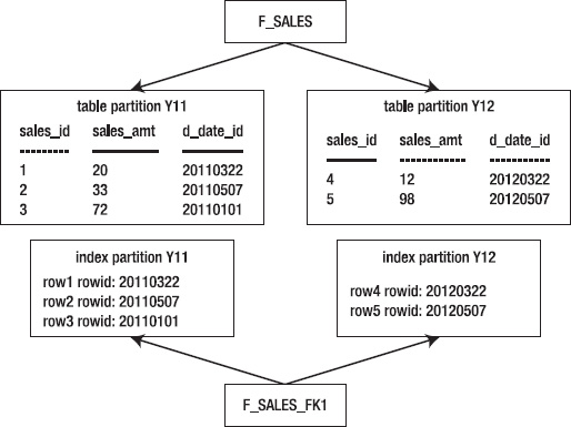
Figure 12–4. Architecture of a locally managed index
If you want the local index partitions to be created in a tablespace (or tablespaces) separate from the table partitions, specify those when creating the index:
create index f_sales_fk1 on f_sales(d_date_id) local

(partition y11 tablespace idx1

,partition y12 tablespace idx2);
Querying USER_IND_PARTITIONS now shows that the index partitions have been created in tablespaces separate from the table partitions:
INDEX_NAME                     PARTITION_ TABLESPACE_NAME

------------------------------ ---------- ---------------

F_SALES_FK1                    Y11        IDX1

F_SALES_FK1                    Y12        IDX2
If you specify the partition information when building a local-partitioned index, the number of partitions must match the number of partitions in the table on which the partitioned index is built.
Oracle automatically keeps local index partitions in sync with the table partitions. You can't explicitly add a partition to or drop a partition from a local index. When you add or drop a table partition, Oracle automatically performs the corresponding work for the local index. Oracle manages the local index partitions regardless of how the local indexes have been assigned to tablespaces.
Local indexes are common in data-warehouse and decision-support systems. If you query frequently by using the partitioned column(s), a local index is appropriate. This approach lets Oracle use the appropriate index and table partition to quickly retrieve the data.
There are two types of local indexes: local prefixed and local nonprefixed. A local-prefixed index is one in which the leftmost column of the index matches the table partition key. The previous example in this section is a local-prefixed index because its leftmost column (D_DATE_ID) is also the partition key for the table.
A nonprefixed-local index is one in which the leftmost column doesn't match the partition key used to partition the corresponding table. For example, this is a local-nonprefixed index:
SQL> create index f_sales_idx1 on f_sales(sales_amt) local;
The index is partitioned with the SALES_AMT column, which isn't the partition key of the table, and is therefore a nonprefixed index. You can verify whether an index is considered prefixed by querying the ALIGNMENT column from USER_PART_INDEXES:
select

 index_name

,table_name

,alignment

,locality

from user_part_indexes

where table_name = 'F_SALES';
Here's some sample output:
INDEX_NAME           TABLE_NAME           ALIGNMENT    LOCALI

-------------------- -------------------- ------------ ------

F_SALES_FK1          F_SALES              PREFIXED     LOCAL

F_SALES_IDX1         F_SALES              NON_PREFIXED LOCAL
You may wonder why the distinction exists between prefixed and nonprefixed. A local-nonprefixed index means the index doesn't include the partition key as a leading edge of its index definition. This can have performance implications, in that a range scan accessing a nonprefixed index may need to search every index partition. If there are a large number of partitions, this can result in poor performance.
You can choose to create all local indexes as prefixed by including the partition-key column in the leading edge of the index. For example, you can create the F_SALES_IDX2 index as prefixed as follows:
SQL> create index f_sales_idx2 on f_sales(d_date_id, sales_amt) local;
Is a prefixed index better than a nonprefixed index? It depends on how you query your tables. You have to generate explain plans for the queries you use and examine whether a prefixed index is able to better take advantage of partition pruning (eliminating partitions to search in) than a nonprefixed index. Also keep in mind that a multicolumn prefixed local index consumes more space and resources than a nonprefixed local index.
Partitioning an Index Differently than Its Table
An index that is partitioned differently than its base table is known as a global index. An entry in a global index can point to any of the partitions of its base table. You can create a global index on any type of partitioned table.
You can create either a range-partitioned global index or a hash-based global index. Use the keyword GLOBAL to specify that the index is built with a partitioning strategy separate from its corresponding table. You must always specify a MAXVALUE when creating a range-partitioned global index. The following example creates a range-based global index:
create index f_sales_gidx1 on f_sales(sales_amt)

global partition by range(sales_amt)

(partition pg1 values less than (25)

,partition pg2 values less than (50)

,partition pg3 values less than (maxvalue));
Figure 12–5 shows that with a global index, the partitioning strategy of the index doesn't correspond to the partitioning strategy of the table.
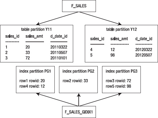
Figure 12–5. Architecture of a global index
The other type of global partitioned index is hash-based. This example creates a hash-partitioned global index:
create index f_sales_gidx2 on f_sales(sales_id)

global partition by hash(sales_id) partitions 3;
In general, global indexes are more difficult to maintain than local indexes. I recommend that you try to avoid using global indexes, and use local indexes whenever possible.
There is no automatic maintenance of global indexes (as there is with local indexes). With global indexes, you're responsible for adding and dropping index partitions. Also, many maintenance operations on the underlying partitioned table require that the global index partitions be rebuilt. The following operations on a heap-organized table render a global index unusable:
ADD (HASH)COALESCE (HASH)DROPEXCHANGEMERGEMOVESPLITTRUNCATE
Consider using the UPDATE INDEXES clause when you perform maintenance operations. Doing so keeps the global index available during the operation and eliminates the need for rebuilding. The downside of using UPDATE INDEXES is that the maintenance operation takes longer due to the indexes being maintained during the action.
Global indexes are useful for queries that retrieve a small set of rows via an index. In these situations, Oracle can eliminate (prune) any unnecessary index partitions and efficiently retrieve the data. For example, global range-partitioned indexes are useful in OLTP environments where you need efficient access to individual records.
Partition Pruning
Partition pruning can greatly improve the performance of queries executing against partitioned tables. If a SQL query specifically accesses a table on a partition key, Oracle only searches the partitions that contain data the query needs (and doesn't access any partitions that don't contain data that the query requires—pruning them, so to speak).
For example, say a partitioned table is defined as follows:
create table f_sales (

 sales_id  number

,sales_amt number

,d_date_id number)

tablespace p1_tbsp

partition by range(d_date_id)(

 partition y10 values less than (20110101)

   tablespace p1_tbsp

,partition y11 values less than (20120101)

   tablespace p2_tbsp

,partition y12 values less than (20130101)

   tablespace p3_tbsp

);
Additionally, you create a local index on the partition-key column:
SQL> create index f_sales_fk1 on f_sales(d_date_id) local;
For this example, insert some sample data:
SQL> insert into f_sales values(1,100,20090202);

SQL> insert into f_sales values(2,200,20110202);

SQL> insert into f_sales values(3,300,20120202);
To illustrate the process of partition pruning, enable the autotrace facility:
SQL> set autotrace trace explain;
Now, execute a SQL statement that accesses a row based on the partition key:
select

 sales_amt

from f_sales

where d_date_id = '20110202';
Autotrace displays the explain plan. Some of the columns have been removed in order to fit the output on the page neatly:
----------------------------------------------------------------------------------

| Id  | Operation                          | Name        |  Rows | Pstart|  Pstop|

----------------------------------------------------------------------------------

|   0 | SELECT STATEMENT                   |             |     1 |       |       |

|   1 |  PARTITION RANGE SINGLE            |             |     1 |     2 |     2 |

|   2 |   TABLE ACCESS BY LOCAL INDEX ROWID| F_SALES     |     1 |     2 |     2 |

|*  3 |    INDEX RANGE SCAN                | F_SALES_FK1 |     1 |     2 |     2 |

----------------------------------------------------------------------------------
In this output, Pstart shows that the starting partition accessed is number 2. Pstop shows that the last partition accessed is number 2. In this example, partition 2 is the only partition used to retrieve data; the other partitions in the table aren't accessed at all by the query.
If a query is executed that doesn't use the partition key, then all partitions are accessed. For example:
SQL> select * from f_sales;
Here's the corresponding explain plan:
----------------------------------------------------------------

| Id  | Operation           | Name    |    Rows| Pstart|  Pstop|

----------------------------------------------------------------

|   0 | SELECT STATEMENT    |         |     3  |       |       |

|   1 |  PARTITION RANGE ALL|         |     3  |     1 |     3 |

|   2 |   TABLE ACCESS FULL | F_SALES |     3  |     1 |     3 |

----------------------------------------------------------------
Notice in this output that the starting partition is number 1 and the stopping partition is number 3. This means partitions 1 through 3 are accessed by this query with no pruning of partitions.
This example is simple but demonstrates the concept of partition pruning. When you access the table by the partition key, you can drastically reduce the number of rows Oracle needs to inspect and process. This has huge performance benefits for queries that are able to prune partitions.
Summary
Oracle provides a partitioning feature that is critical for implementing large tables and indexes. Partitioning is vital for building highly scalable and maintainable applications. This feature works on the concept of logically creating an object (table or index) but implementing the object as several separate objects. A partitioned object allows you to build, load, maintain, and query on a partition-by-partition basis. Maintenance operations such as deleting, archiving, updating, and inserting data are manageable because you're working on only a small subset of the large logical table.
If you work in data-warehouse environments or with large databases, you must be highly knowledgeable of partitioning concepts. As a DBA, you're required to create and maintain partitioned objects. You have to make recommendations about table-partitioning strategies and where to use local and global indexes. These decisions have a huge impact on the usability and performance of the system.
After this chapter, the book focuses on utilities used to copy and move users, objects, and data from one environment to another. Oracle's Data Pump and External Table feature are covered in the next two chapters.