
In the last chapter, I talked about how data science tasks may encounter a wide variety of dataset sizes, ranging from kilobytes to petabytes. There can be a range of scale either in the number of samples or the extent of feature dimensionality. To handle complex data analytics and machine learning, data scientists employ a dizzying array of models, and that ecosystem scales up quickly, too.
Handling data and models at scale is a special skill to be acquired. When a data scientist starts learning the tradecraft, they first focus on understanding the mathematical basis, data wrangling and formatting concepts, and how to source and scrape data from various sources. In the next stage, they focus mainly on various ML algorithms and statistical modeling techniques and how to apply them for various tasks. Model performance and hyperparameter tuning remains their sole focus.
However, in almost all real-life scenarios, the success of a data science pipeline (and its value addition to the overall business of the organization) may depend on how smoothly and flawlessly it can be deployed at scale (i.e., how easily it can handle large datasets, faster streaming data, rapid change in the sampling or dimensionality, etc.). In this era of Big Data, the principles of the five V’s (or six) must be embraced by enterprise-scale data science systems.
Of course, a single data scientist will not oversee implementing this whole enterprise or the pipeline. However, knowledge about scaling up the data science workflow is fast becoming a prerequisite for even an entry-level job in this field. There are a few different dimensions to that knowledge: cloud computing, Big Data technologies like Hadoop and Spark, and parallel computing with data science focus, for example.
The topics of cloud computing and associated tools (think AWS, Google Cloud Service, or Azure ML) are squarely beyond the scope of this book. Additionally, there are excellent resources (both online courses and textbooks) for learning the essentials of distributed data processing with the Hadoop infrastructure and related technologies. This chapter focuses on the Python-based parallel computing aspects that can be used directly for data science tasks. Much like the last chapter, I will discuss some of the limitations that arise while doing analysis with large and complex datasets using the most common data analysis and numerical computing libraries like pandas or NumPy and discuss alternative libraries to help with those tasks.
It is to be noted, however, that this is not going to be an exhaustive discussion about general parallel computing tricks and techniques with Python. In fact, I will avoid detailed treatment of the topics that often come up in a standard Python parallel computing tutorial or treatise, such as working with built-in modules like multiprocessing, threading, or asynco. The focus, like any other chapter in this book, is squarely on data science, and therefore, I will cover two libraries named Dask and Ray that truly add value to any data science pipeline where you want to mix the power of parallel computing.
Parallel Computing for Data Science
You are highly likely to get a response like 4 or 6. This is because all modern CPUs consist of more than one core; they’re parallel computing units, effectively. There are subtle differences between the actual physical cores (electronic units with those nanometer-scale transistors) and logical cores, but for all computing purposes, you can think of the logical cores as the fundamental units in your system.
So, we have multiple cores, and we should be able to take advantage of that hardware design in our data science tasks. What might that look like?
Single Core to Multi-Core CPUs
Although this is a book about data science, sometimes it is necessary (and nostalgic) to take a slight detour into the hardware realm and revisit the history of development on that side. For parallel computing, a lot of hardware development had to happen over a long period of time before the modern software stack started taking full-blown advantage of that development. It will be beneficial to get a brief glimpse of this history to put our discussion in context.
The earliest commercially available CPU was the Intel 4004, a 4-bit 750kHz processor released in 1971. Since then, processor performance improvements were mainly due to clock frequency increases and data/address bus width expansion. A watershed moment was the release of the Intel 8086 in 1979 with a max clock frequency of 10MHz and a 16-bit data width and 20-bit address width.
The first hint of parallelism came with the first pipelined CPU design for the Intel i386 (80386) which allowed running multiple instructions in parallel. Separating the instruction execution flow into distinct stages was the key innovation here. As one instruction was being executed in one stage, other instructions could be executed in the other stages and that led to some degree of parallelism.
At around the same time, superscalar architecture was introduced. In a sense, this can be thought of as the precursor to the multi-core design of the future. This architecture duplicated some instruction execution units, allowing the CPU to run multiple instructions at the same time if there were no dependencies in the instructions. The earliest commercial CPUs with this architecture included the Intel i960CA, AMD 29000 series, and Motorola MC88100.
The unstoppable march of Moore’s Law (shrinking the transistor sizes and manufacturing cost at an exponential pace; www.synopsys.com/glossary/what-is-moores-law.html) helped fuel this whole revolution in microarchitecture with the necessary steam. Semiconductor process technology was improving and lithography was driving the transistor nodes to the realm of sub 100 nm (1/1000th of the width of a typical human hair), supporting circuitry, motherboards, and memory technology (taking advantage of the same manufacturing process advancements).
The war for clock frequency heated up and AMD released the Athlon CPU, hitting the 1GHz speed for the first time, at the turn of the century in 1999. This war was eventually won by Intel, who released a dizzying array of high-frequency single-core CPUs in the early 2000s, culminating in the Pentium-4 with a base frequency around 3.8GHz - 4GHz.
But fundamental physics struck back. High clock frequencies and nanoscale transistor sizes resulted in faster circuit operations, but the power consumption shot up as well. The direct relationship between frequency and power dissipation posed an insurmountable problem for scaling up. Effectively, this power dissipation resulted in so-called higher leakage current that destabilized the entire CPU and system operation when the transistor count was also going up into billions (imagine billions of tiny and unpredictable current leakages happening inside your CPU).
To solve this issue, multi-CPU designs were tried that housed two physical CPUs sharing a bus and a common memory pool on a motherboard. The fundamental idea is to stop increasing the frequency of operations and go parallel by distributing the computing tasks over many equally powerful computation units (and then accumulate the result somehow). But due to communication latencies from sharing external (outside the package) bus and memory, they were not meant to be truly scalable designs.
Fortunately, true multi-core designs followed soon after where multiple CPU cores were designed from the ground up within the same package, with special consideration for parallel memory and bus access. They also featured shared caches that are separate from the individual CPU caches (L1/L2/L3) to improve inter-core communication by decreasing latency significantly. In 2001, IBM released Power4, which can be considered the first multi-core CPU, although the real pace of innovation and release cycle picked up after Intel’s 2005 release of the Core-2 Duo and AMD’s Athlon X2 series.
Many architectural innovations and design optimizations are still ongoing in this race. Enhancing core counts per generation has been the mainstay for both industry heavyweights, Intel and AMD. While today’s desktop workstation/laptops regularly use 4 or 6 core CPUs, high-end systems (enterprise data center machines or somewhat expensive cloud instances) may feature 12 or 16 cores per CPU.
For the data science revolution and progress, it makes sense to follow this journey closely and reap the benefits of all the innovations that hardware design can offer. But it is easier said than done. Parallelizing everyday data science tasks is a non-trivial task and needs special attention and investment.
What Is Parallel in Data Science?
For data science jobs, both data and models are important artifacts. Therefore, one of the first considerations to be made for any parallel computing effort is to the focal point of parallelizing: data or model.
Why do you need to think this through? Because some artifacts are easier to be imagined to be parallelized than the others. For example, assume you have 100 datasets to run some statistical testing on and 4 CPU cores in your laptop. It is not hard to imagine that it would be great if somehow you could distribute the datasets evenly across all the cores and execute the same code in parallel (Figure 10-1). This should reduce the overall time to execute the statistical testing code significantly, even if the scheme involves some upfront overhead for dividing and distributing data, and some end-of-the-cycle aggregation or accumulation of the processed data.

Distributing datasets across multiple computing cores
Moreover, data science is not limited to model exploration and statistical analysis on a single person’s laptop (or a single cloud-based compute node) anymore. From a single machine (however powerful it might be), the advantages are apparent for large-scale data analytics when one connects to a cluster architecture consisting of multiple computers banded together with high-speed network. In the limiting case, such a cluster aims to become a single entity of computing for all intents and purposes: a single brain arising out of parallel combination and communication among many smaller brains.
Naturally, data scientists start imagining all kinds of possibilities that can be tried and tested with this collective brain. Alongside splitting a large collection of datasets, they can think of splitting models (or even modeling subtasks) into chunks and executing them in a parallel fashion. Datasets can be sliced and diced in multiple ways and all those dimensions might be parallelized, depending on the problem at hand. Some tasks may benefit from splitting data samples in rows; others may benefit from column-wise splitting.

Cluster of computing nodes for parallelizing data science tasks in various dimensions: data, model, optimizations, and so on
Parallel Data Science with Dask
Dask is a feature-rich, easy-to-use, flexible library for parallelized and scalable computing in the Python ecosystem. While there are quite a few choices and approaches for such parallel computing with Python, the great thing about Dask is that it is specifically optimized and designed for data science and analytics workloads. In that way, it really separates itself from other major players such as Apache Spark.
In a typical application scenario, Dask comes to the rescue when a data scientist is dealing with large datasets that would have been tricky (if not downright impossible) to handle with the standard Python data science workflow of NumPy/ pandas/scikit-learn/TensorFlow. Although these Python libraries are the workhorses of any modern data science pipeline, it is not straightforward how to take advantage of large parallel computing infrastructure or clusters with these libraries.
At the minimum, one must spend quite a bit of manual effort and set up customized code or preprocessing steps to optimally distribute a large dataset or split a model that can be executed on the parallel computing infrastructure. Moreover, this limitation is not only for cloud-based clusters but applies to a single machine scenario as well. It is not apparent how to take advantage of all the logical cores or threads of a powerful workstation (with a single standalone CPU) when doing a pandas data analysis task or using SciPy for a statistical hypothesis testing. Some of the design features of these libraries may even fundamentally prevent us from using multiple CPU cores at once.
Fortunately, Dask takes away the pain of planning and writing customized code for turning most types of data science tasks into parallel computing jobs and abstracts away the hidden complexity as much as possible. It also offers a DataFrame API that looks and feels much like the pandas DataFrame so that standard data analytics and data wrangling code can be ported over with minimal change and debugging. It also has a dedicated ML library (APIs similar to that of scikit-learn). Let’s explore how Dask works and more features in the next sections.
This article (https://coiled.io/is-spark-still-relevant-dask-vs-spark-vs-rapids/) lays out the similarities and differences nicely. In brief, Dask is more “friendly and familiar” to data scientists working with Python codebase and solving problems that do not always restrict themselves to SQL-type data queries.
How Dask Works Under the Hood

Dask client-scheduler-worker operations under the hood
Dask array
Dask DataFrame
Dask bag
Dask task graph
Dask Array
This is an implementation of a subset of the NumPy n-dimensional array (or ndarray) interface using blocked algorithms that effectively cut up a large array into many small arrays/chunks. This facilitates computation on out-of-core (larger than memory) arrays using all the cores in a computer in a parallel fashion. These blocked algorithms are coordinated using Dask task graphs. For more details on Dask arrays, go to the official documentation at https://docs.dask.org/en/latest/array.html.
Dask DataFrame
Essentially, a Dask DataFrame is a large-scale parallelized DataFrame composed of many smaller pandas DataFrames, split along the index. Depending on the size and situation, the pandas DataFrames may exist on the disk for out-of-core computing on a single machine, or they may live on many different computing nodes in a cluster. A single Dask DataFrame operation triggers many operations down the chain (i.e., on the constituent pandas DataFrames in a parallel manner).

The pandas official documentation suggests using Dask for large datasets
Dask Bag
This is a data structure that implements operations like map, filter, fold, and groupby on collections of generic Python objects like lists or tuples. It uses a small memory footprint using Python iterators and is inherently parallelized.
Apache Spark has its famous Resilient Distributed Dataset (RDD; https://databricks.com/glossary/what-is-rdd). A Dask Bag is a Pythonic version of that RDD, suitable for operations inherently popular with users of the Hadoop file system. They are mostly used to parallelize simple computations on unstructured or semi-structured data such as text data, JSON records, log files, or customized user-defined Python objects.
Dask Task Graph
Dask uses the common approach to parallel execution in user-space: task scheduling. With this approach, it breaks the main high-level program/code into many medium-sized tasks or units of computation (e.g., a single function calls on a non-trivial amount of data). These tasks are represented as nodes in a graph. Edges run between nodes if one task is dependent on the data produced by another. A task scheduler is called upon to execute this whole graph in a way that respects all the inter-node data dependencies and leverages parallelism wherever possible, thereby speeding up the overall computation.

Dask uses a full task scheduling approach for its task graph

Dask collections, task graph, and schedulers
Works on Many Types of Clusters
Hadoop/Spark clusters running YARN
HPC clusters running job managers like SLURM, SGE, PBS, LSF, or others
common in academic and scientific labs
Kubernetes clusters
This makes Dask a truly powerful engine for parallel computing no matter the underlying distributed data processing infrastructure choice. Naturally, Dask code and pipelines can be easily ported from one organization to another or shared among the teams of a large data science organization.
Basic Usage Examples
Here is how you can define and examine some of the data structures you just learned about. Let’s start with arrays and then go on to show some examples with DataFrames and Bags.
Almost all the code snippets in this chapter are for illustration and conceptualization purpose only. They are not fully executable, working code. The reason for this is brevity. The book focuses on concepts and learning and does not intend to act as a code manual. Working code examples are provided in the accompanying Jupyter notebooks (or GitHub links).
Array

A 2D Dask array created from a NumPy array of random numbers

A 3D Dask array created from a NumPy array of random numbers

A simple summation operation leads to a new array and task graph

Determining the max out of the summed values along columns

Final computation for the 3D array

A high-level task graph for the sum-max operations
In the Jupyter notebook, each of these layers can be expanded to see more details. You are encouraged to check out the accompanying notebook.
DataFrames

A time series DataFrame in Dask showing the data schema

A Dask DataFrame showing the first few entries

Time series resampled data mean

Accesing and computing the data for a particular day/partition
Dask Bags

Dask bag containing JSON records (the first two records are shown here)

Filtering operation done on the records contained in the Dask Bag
There are many powerful usages for Dask Bags with semi-structured datasets that would have been difficult to accomplish just with an array or DataFrames.
Dask Distributed Client
All the usage examples in the earlier sections feature the formalism and lazy evaluation nature of Dask APIs (arrays, DataFrames, and Bags), but they don’t showcase the distributed/parallelized nature of computation in an obvious manner. For that, you must select and use the distributed scheduler from the Dask repertoire. It is actually a separate module or lightweight library called Dask.distributed that extends both the concurrent.futures and Dask APIs to moderate sized clusters.
Low overhead and latency: There is only about 1ms of overhead for each task. A small computation and network roundtrip can be completed in less than 10ms.
Data sharing between peers: Worker nodes (e.g., logical cores on a local machine or cheap computing nodes in a cluster) communicate with each other to share data.
Locality of the data: Computations happen where the data lives. Scheduling algorithms distribute and schedule tasks following this principle. This also minimizes network traffic and improves the overall efficiency.
Complex task scheduling: This is probably the most attractive feature. The scheduler supports complex workflows and is not restricted to standard map/filter/reduce operations that are the primary feature of other distributed data processing frameworks like Hadoop-based systems. This is absolutely necessary for sophisticated data science tasks involving n-dimensional arrays, machine learning, image or high-dimensional data processing, and statistical modeling.
The flexibility and power of the scheduler also stems from the fact that it is asynchronous and event driven. This means it can simultaneously respond to computation requests from multiple clients and track the progress of a multitude of workers that have been given tasks already. It is also capable of concurrently handling a variety of workloads coming from multiple users while also managing a dynamic worker population with possible failures and new additions.
The best thing for the user, a data scientist, is that they can use all these features and powers with pure Python code and a minimal learning curve. Cluster management or distributed scheduling is not a trivial matter to accomplish programmatically. A data scientist using Dask does not have to bother about those complexities as they are abstracted away. That’s where the theme of productive data science gets its support from libraries like Dask.

Starting up a Dask-distributed cluster/scheduler (on a local machine)
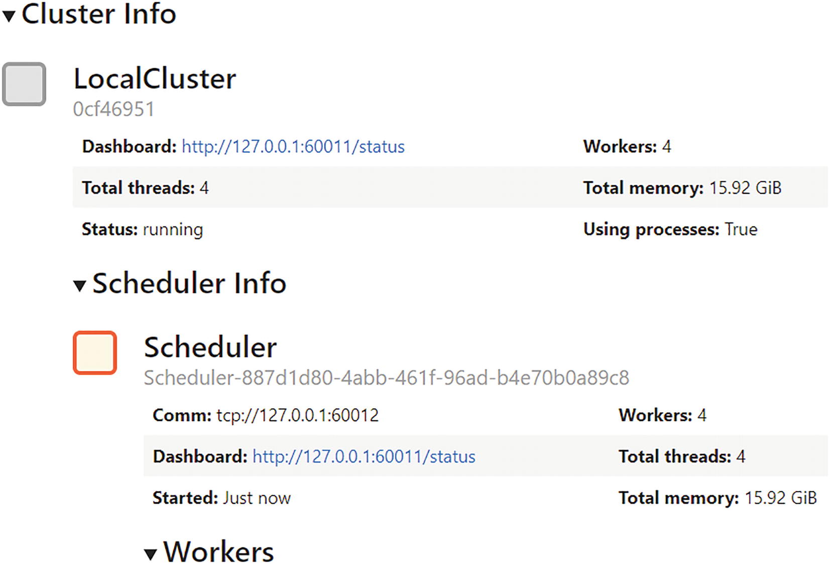
Cluster and scheduler info for Dask distributed client setup
address: IP address (with port) of a real cloud-based, remote cluster or the local host machine. If you can afford to rent a high-end cloud instance with a high CPU count (as discussed in the previous chapter), the Dask scheduler can directly connect to it and start utilizing the resources. When not specified, only the local host machine is taken up as the computing node.
n_workers: Explicitly specifying the number of CPU cores that the cluster will be able to use. This could be important for resource constrained situations or if there are many Dask tasks to be distributed among a finite number of CPU cores.
threads_per_worker: Just like specifying number of CPU cores, this dictates the number of threads per core. Generally, this number is 1 or 2.
memory_limit: This is another useful keyword to use for optimally managing the total system memory for the distributed client. This limit is on a per-CPU core basis and should be a string (e.g., ‘2 GiB’).
Once the scheduler is started up, it manages the distributed computing aspects by itself. However, there is a certain way to submit jobs to the scheduler using map and submit methods. Here is a (somewhat contrived) example.
A synthetic batch of data for which a distributed processing needs to be run
21 max computation (from 1,000 data points each time)
21 median computation (from 1,000 data points each time)
Two arithmetic mean computations (of 21 max/median values each time)
A final difference calculation
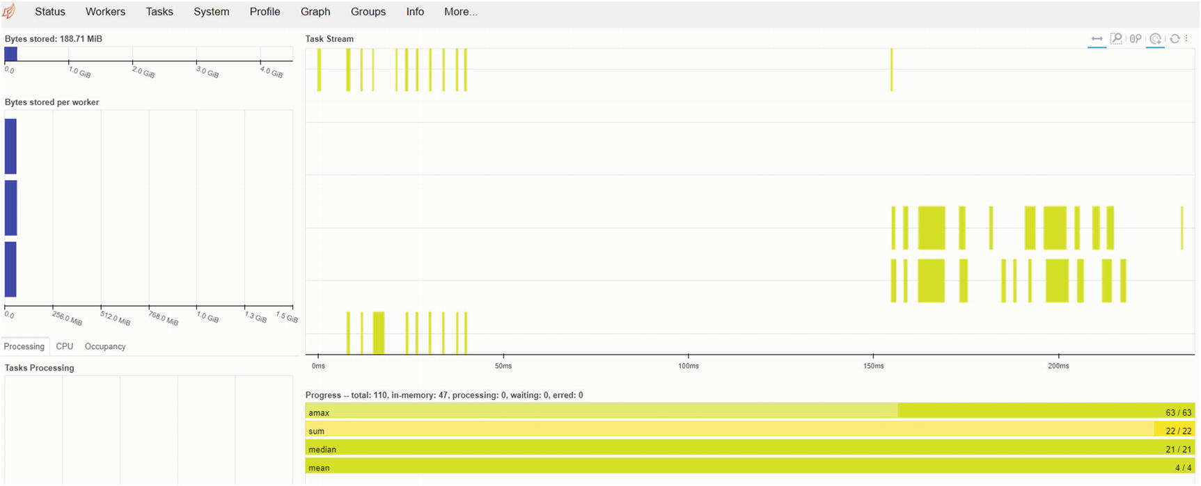
Task status view of the dynamic Dask dashboard
This is a static snapshot of the task status tab of the dashboard. When the parallel processes execute (distributed over multiple CPU cores), the graph changes and updates dynamically as all the data chunks are split and shared among workers. A good visual demonstration of this dynamic process can be seen in an article that I published at https://medium.com/productive-data-science/out-of-core-larger-than-ram-machine-learning-with-dask-9d2e5f29d733 with a hands-on example involving the Dask Machine Learning library. You are encouraged to check out this article.

Workers information view of the dynamic Dask dashboard
Dask Machine Learning Module
While Dask provides an amazing suite of parallel and out-of-core computing facilities and a straightforward set of APIs (Arrays, DataFrames, Bags, etc.,), the utility does not stop there. Going beyond the data wrangling and transformation stage, when data scientists arrive at the machine learning phase, they can still leverage Dask for doing the modeling and preprocessing tasks with the power of parallel computing. All of this can be achieved with a minimal change in their existing codebase and in pure Pythonic manner.
For ML algorithms and APIs, Dask has a separately installable module called dask-ml. Full treatment of that module is beyond the scope of this book. You are again encouraged to check out the above-mentioned article to get a feel about the API. Here, I will briefly discuss some key aspects of dask-ml.
What Problems Does It Address?
Fundamentally, libraries like dask-ml addresses the dual problems of data scaling and model scaling.
The data scaling challenge comes about with the Big Data domain, for example, when the computing hardware starts having trouble containing training data in the working memory. So, this is essentially a memory-bound problem. Dask solves this problem by spilling data out-of-core onto drive storage and providing incremental meta-learning estimators that can learn from batches of data rather than having to load entire dataset in the memory.
The model scaling challenge, on the other hand, raises its ugly head when the parametric space of ML model becomes too large and the operations become compute-bound. To address these challenges, you can continue to use the efficient collections Dask offers (arrays, DataFrames, bags) and use a Dask Cluster to parallelize the workload on an array of machines. Even the task of parallelization has choices. It can occur through one of the built-in integrations (e.g., Dask’s joblib back end to parallelize scikit-Learn directly) or one of dask-ml estimators (e.g., a hyper-parameter optimizer or a parallelized Random Forest estimator).
Tight Integration with scikit-learn
Following through the principle of simplicity of use, dask-ml maintains a high degree of integration and the drop-in replacement philosophy with the most popular Python ML library, scikit-learn. Dask-ml provides data preprocessing, model selection, training, and even data generating functions just like scikit-learn does while supporting Dask collections as native objects to use with those APIs.
It is easy to spot the almost line-by-line similarity between this code and a standard scikit-learn pipeline. This is called the drop-in replacement ability of dask-ml. You may also notice the use of the Parquet file format for reading a large dataset efficiently (into a Dask DataFrame) from a disk drive or network storage. You may check out my article on this topic (https://medium.com/productive-data-science/out-of-core-larger-than-ram-machine-learning-with-dask-9d2e5f29d733). When executed, this code combines the advantage of out-of-core data handling of a Dask DataFrame with the parallelized estimator API and delivers a scalable machine learning experience for the data scientist, thereby boosting their productivity.
In the code above, note that the main estimator comes from scikit-learn itself. The Dask part is only a wrapper that utilizes the underlying estimator to work on a Dask collection like a DataFrame for lazy evaluation and out-of-core computing.
Parallel Computing with Ray
Parallel computing in pure Python has recently been revolutionized by the rapid rise of a few great open-source frameworks, Ray being one of them. It was created by two graduate students in the UC Berkley RISElab (https://rise.cs.berkeley.edu/), Robert Nishihara and Philipp Moritz, as a development and runtime framework for simplifying distributed computing. Under the guidance of Professors Michael Jordan and Ion Stoica, it rapidly progressed from being a research project to a full-featured computing platform with many subcomponents built atop it for different AI and ML focused tasks (hyperparameter tuning, reinforcement learning, data science jobs, and even ML model deployment).
Currently, Ray is maintained and continuously enhanced by Anyscale (www.anyscale.com/), a commercial entity (startup company) formed by the creators of Ray. It is a fully managed Ray offering that accelerates building, scaling, and deploying AI applications on Ray by eliminating the need to build and manage complex infrastructure.
Features and Ecosystem of Ray
Ray achieves scalability and fault tolerance by abstracting the control state of the system in a global control store and keeping all other components stateless.
It uses a shared-memory distributed object store to efficiently handle large data through shared memory, and it uses a bottom-up hierarchical scheduling architecture to achieve low-latency and high-throughput scheduling.
Ray presents a lightweight API based on dynamic task graphs and actors to express a wide range of data science and general-purpose applications in a flexible manner.

Distributed data science/ML ecosystem built atop Ray
In this section, I will show only a couple of examples of running parallel data science workloads using Ray. You are highly encouraged to check out the official documentation (www.ray.io/docs) and try out all the great features that this library provides.
Simple Parallelization Example
Before I show the hands-on examples, I want to mention that Ray is currently built and tested for Linux and Mac OS, and the Windows version is experimental and not guaranteed to be stable. Therefore, you are encouraged to practice Ray examples in a Linux environment or create a virtual machine (VM) on your Windows platform, install Ray, and continue.

Multiple logical CPU cores assigned to a VM that is used to run Ray

Snapshot of a Ray dashboard (with five CPU assignments)

Pipeling sub-components in the correct order
Ray Dataset for Distributed Loading and Compute
Ray Datasets (https://docs.ray.io/en/latest/data/dataset.html) are the standard (and recommended) way to load and exchange data in the Ray ecosystem. These objects provide basic distributed data transformations such as map, filter, and repartition, and play well with a wide variety of file formats, data sources, and distributed frameworks for easy loading and conversion. They are also specifically designed to load and preprocess data with high performance for distributed ML training pipelines built with Ray such as Ray-Train. (https://docs.ray.io/en/latest/train/train.html#train-docs).
and are available as Beta from Ray 1.8+ version onwards. If you are using an older version of Ray, you need to upgrade to take advantage of them. Also, make sure that the PyArrow library is installed.
Ray Datasets are a good candidate for the last-mile data processing blocks (before data is fed into a parallelized ML task flow) where the initial data sources are traditional RDBMS, output of ETL pipeline, or even Spark DataFrames.
Previously, I talked about Apache Arrow and how these modern data storage formats are revolutionizing the data science world. Ray Datasets, at their core, implement distributed Arrow. Each Dataset is essentially a list of Ray object references to blocks that hold Arrow tables (or Python lists in some cases). The presence of such block-level structure allows the parallelism and compatibility with distributed ML training. In this manner, Ray Datasets are similar to what you saw with Dask. Moreover, since Datasets are just lists of Ray object references, they can be freely (almost no memory operation overhead) exchanged between Ray tasks, actors, and libraries. This lets you have tremendous flexibility with their usage and integration, and it improves the system performance.

Snapshot of Ray Datasets’ input compatibility
So, by default, it has created 200 blocks of object reference and also assigned a schema of integer to the data. This parallelism and data type integration inherently makes the Dataset more efficient than traditional data sources like pandas DataFrame.
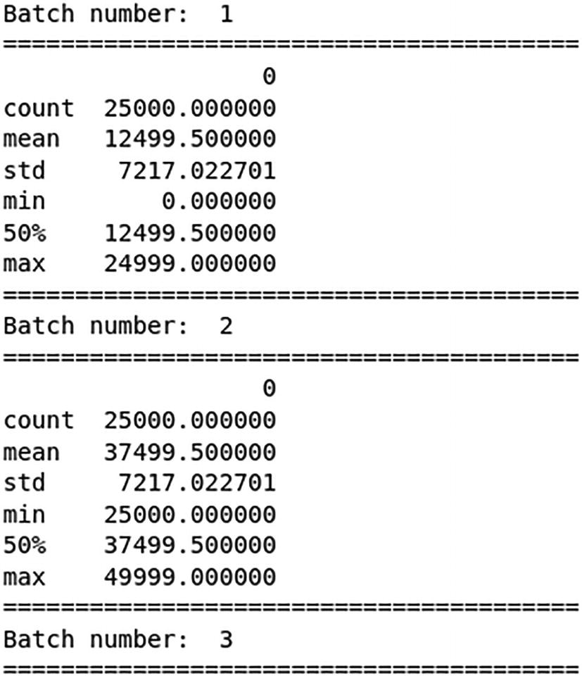
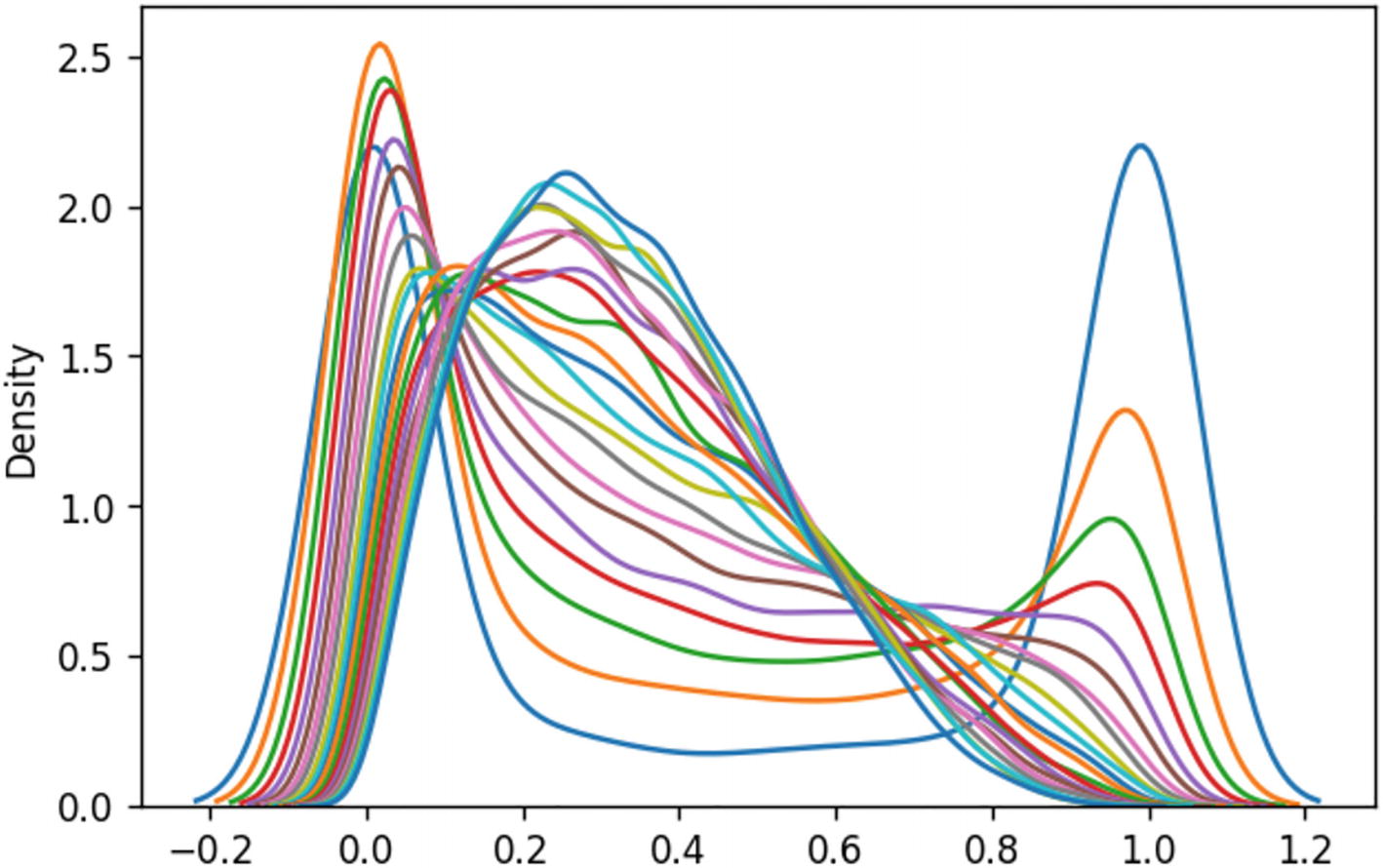
Partial result of batch iteration of a Ray Dataset as chunks of a pandas DataFrame
Summary
In this chapter, I continued the discussion about making data science scalable across large datasets and models with parallel (and distributed) computing tools. I discussed that both raw data and large models can be processed with these parallel processing techniques. With the advent of modern multi-core CPUs and the easy availability of large computing clusters at a reasonable cost (from cloud vendors), the prospects of parallelized data science look bright.
I focused particularly on two Python frameworks, Dask and Ray. I covered, in detail, various core data structures and internal representations that Dask provides to make parallel computing easy and fun. I also discussed the Dask distributed client in detail with hands-on examples. For Ray, I covered the basic Ray parallelism with special decorators and methods and the distributed data loading functionalities.
In the next chapter, I will go beyond the realm of the CPU and venture into a different kind of scalability: how to port and take advantage of GPU-based systems for data science tasks.