Example of a Productive DL Task Flow

Deep learning makes it easy to train ML models for highly nonlinear (and even noisy) datasets and phenomena. Modern frameworks like Keras/TensorFlow/PyTorch offer powerful and flexible APIs to build these models with relative ease and a surprisingly small amount of code. However, an end-to-end DS flow can be made much more productive if you follow some simple guidelines on how you build, manage, and utilize DL code. An approach of building compact modules and a systematic flow (shown in Figure 5-1) can help. Some examples of related guidelines are discussed below in the form of questions.

• One of the most common and repetitive tasks for DL analysis is to build out a deep neural network (DNN) object. Data scientists routinely use non-modularized code to just add layers (e.g., from Keras (https://keras.io/api/layers/) or PyTorch https://pytorch.org/tutorials/recipes/recipes/defining_a_neural_network.html) APIs) and build this as a local variable in their Jupyter notebook. Wouldn’t it be a much better idea to create a custom function for this task?

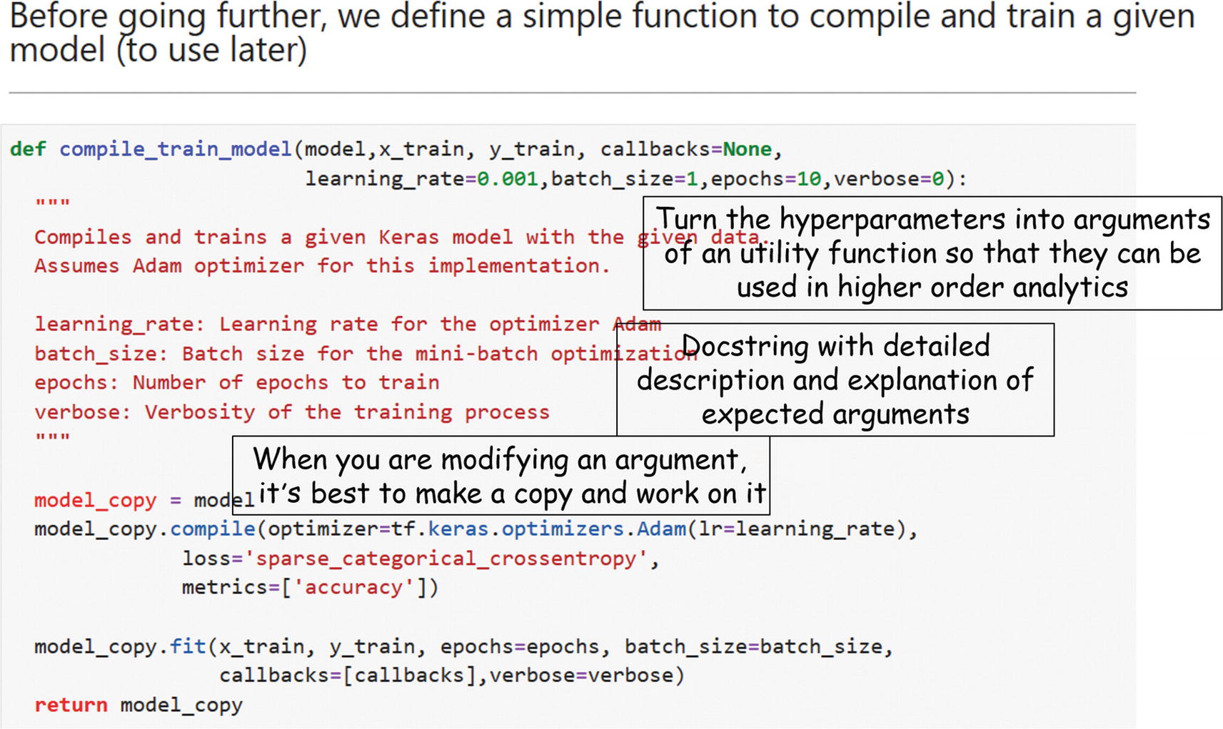
• After building an (untrained) model, you must compile (set learning rate, batch size, etc.) and run the model with data. Would a custom function help make this task modularized as well?

• When you make such a DNN builder function, which parameters will be passed on? Which ones can be optional? What are the default values? If you encounter a situation where you don’t know how many parameters need to be passed on, are you using the *args and **kwargs that Python offers?

• Did you write a docstring for that function to let others know what the function does and what parameters it expects plus an example?

• Can you also modularize the code used to create the visual analytics based on the output of those model functions?

Wrappers, Builders, Callbacks

Fundamentally, in the subsection above I described wrapping up the most essential tasks in a DL-based workflow inside custom functions and using them as the core building blocks of your data science code. Additionally, you can wrap up the tasks related to data formatting/transformation and prediction/inference in a similar fashion.

It is to be noted that wrapper functions for regression and classification tasks can have separate sets of architecture and parameters. So, it makes sense to keep their build customized. The choice of the default parameter values in the wrapper functions is of critical importance, too.

Finally, if you want to extend this approach all the way to the full OOP paradigm, you can build out classes and utility modules incorporating all these wrappers as special methods. You can call this a DL utility module, which you can call upon in any data science task where supervised ML modeling is needed.

Business/Data Science Question

The basic ML task for this dataset seems straightforward. But what if there is a higher-order optimization or visual analytics question around this core ML task: how does the model architecture complexity impact the minimum epochs it takes to reach the desired accuracy?

It should be clear to you why we even bother about such a question: because this is related to the overall business optimization. Training a neural net is not a trivial computational matter (www.technologyreview.com/s/613630/training-a-single-ai-model-can-emit-as-much-carbon-as-five-cars-in-their-lifetimes/). Therefore, it makes sense to investigate what minimum training effort must be spent to achieve a target performance metric and how the choice of architecture impacts it.

The image classification accuracy could be related to a broader business outcome such as a fashion recommendation or clothing identification in a store. The core data science task helps optimize the cost of running that business task—to use the image database with the optimal expenditure of computing resources using the ML code as the underlying nuts and bolts.

In this example, you will not even use a convolutional neural network (CNN; https://towardsdatascience.com/a-comprehensive-guide-to-convolutional-neural-networks-the-eli5-way-3bd2b1164a53), which are commonly used for image classification tasks. This is because, for this dataset, a simple densely connected neural net can accomplish reasonably high accuracy, and, in fact, a sub-optimal performance is required to illustrate the main point of the higher-order optimization question posed above.

Inherit from the Keras Callback

You inherit a Keras callback class (as the base) and write your own subclass by adding a method that checks the training accuracy and takes an action based on that value. The code snapshot and some explanations are shown in Figure 5-3. More details on this can be found in the official TensorFlow article “Writing your own callbacks” at www.tensorflow.org/guide/keras/custom_callback.

Basically, this simple callback results in dynamic control of the epochs; the training stops automatically when the accuracy reaches the desired threshold. Figure 5-4 shows a snapshot of an example run.

Model Builder and Compile/Train Functions

Next, you put the Keras model construction code in a utility function so that a model of an arbitrary number of layers and architecture (as long as they are densely connected) can be generated using simple user input in the form of some function arguments. The code snapshot and the associated explanations are shown in Figure 5-5.

You also put the compilation and training code into a utility function to use those hyperparameters in a higher-order optimization loop conveniently. The code snapshot and the associated explanations are shown in Figure 5-6.

Visualization Function

Next, it’s time for visualization. Generic plot functions take raw data as input. However, if you have a specific purpose of plotting the evolution of training set accuracy (and showing how it compares to the target), then your plot function should just accept the (trained) deep learning model as the input and generate the desired plot. The code snapshot and the associated explanations are shown in Figure 5-7.

A typical result (loss-accuracy plot) is shown in Figure 5-8.

Final Analytics Code, Compact and Simple

Thus far you have modularized the core DL code. Now you can take advantage of all the functions and classes you defined earlier and bring them together to accomplish the higher-order optimization task. Consequently, your final code will be highly compact, but it will generate the same interesting plots of loss and accuracy over epochs for a variety of accuracy threshold values and DNN architectures (neuron counts).

This will give you the ability to use a minimal amount of code to produce visual analytics about the choice of performance metric (classification accuracy in this case) and DNN architecture. This is the first step towards building an optimized machine learning system.

This code generates the cases shown in Figure 5-9.

The final analytics/optimization code is succinct and easy to follow for a high-level user who does not need to know the complexity of Keras model building or callbacks classes. This is the core principle behind OOP, the abstraction of the layers of complexity, which you are able to accomplish for your deep learning task.

Some representative results are shown in Figure 5-10; they are automatically generated by executing the code block above. It clearly shows how with a minimal amount of high-level code you can generate visual analytics to judge the relative performance of various neural architectures for various levels of performance metrics. This enables a user, without tweaking the lower-level functions, to easily make a judgment on the choice of a model as per the desired accuracy and complexity.

Also, note the custom titles for each plot. These titles clearly enunciate the target performance and the complexity of the neural net, thereby making the analytics easy. It was a small addition to the plotting utility function, but this shows the need for careful planning while creating such functions. If you had not planned for such an argument to the function, it would not have been possible to generate a custom title for each plot. This careful planning of the API (application program interface) is part and parcel of good OOP.

Turn the Scripts into a Utility Module

So far, you may be working with a Jupyter notebook, but you may want to turn this exercise into a neat Python module that you can import from any time you want. Just like you write from matplotlib import pyplot, you can import these utility functions (Keras model build, train, and plotting) anywhere. The idea is shown in Figure 5-11.

Summary of Good Practices

You just learned some good practices, borrowed from OOP, to apply to a DL analysis task. Almost all of them may seem trivial to seasoned software developers. However, this chapter is designed for budding data scientists who may not have that structured programming background but need to understand the importance of imbuing these good practices in their ML workflow.

In the next chapter, you will try your hand at building your own ML estimator class based on these principles. For a taste of DL utility functions and a neural net trainer class, please read “Deep learning with Python” at https://github.com/tirthajyoti/Deep-learning-with-Python/tree/master/utils.

The Dataset

For each class, there are about 800 photos. The photos are not particularly high resolution (about 320 x 240 pixels each). They are not reduced to a single size since they have different proportions. However, they come organized neatly in five directories named with the corresponding class labels. You can take advantage of this organization and apply the Keras methods to streamline the training of your convolutional network.

The full Jupyter notebook is in the GitHub repository. I will use selected snapshots of the code in this section to show the important parts for illustration.

For illustration, Figure 5-13 shows how they are stored on a local hard disk. Some sample images are in Figure 5-14.

Building the Data Generator Object

This is where the actual magic happens. The official description of the ImageDataGenerator class says "Generate batches of tensor image data with real-time data augmentation. The data will be looped over (in batches)."

Basically, it can be used to augment image data with a lot of built-in preprocessing such as scaling, shifting, rotation, noise, whitening, etc. Right now, you’ll just use the rescale attribute to scale the image tensor values between 0 and 1. Here is a useful article on this aspect of the class: “How to increase your small image dataset using Keras ImageDataGenerat​or”(https://medium.com/@arindambaidya168/https-medium-com-arindambaidya168-using-keras-imagedatagenerator-b94a87cdefad).

But the real utility of this class for the current demonstration is the super useful method named flow_from_directory, which can pull image files one after another from the specified directory. Note that this directory must be the top-level directory where all the subdirectories of individual classes can be stored separately. The flow_from_directory method automatically scans through the subdirectories and sources the images along with their appropriate labels.

You can specify the class names (as you did here with the classes argument) but this is optional. However, you will later see how this can be useful for selective training from a large trove of data.

Another useful argument is the target_size, which lets you resize the source images to a uniform size of 200 x 200, no matter the original size of the image. This is some cool image-processing right there with a simple function argument.

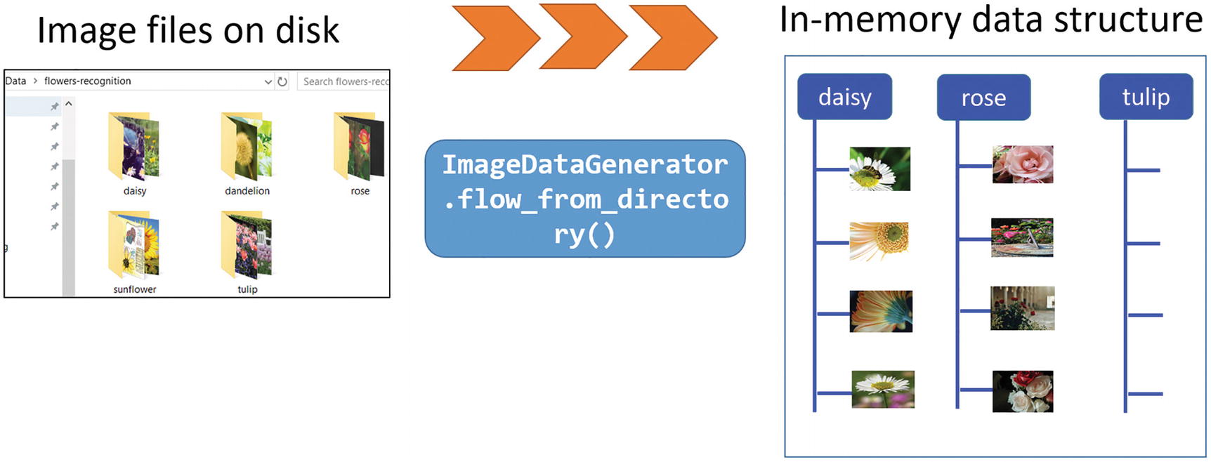
When you run this code, the Keras function scans through the top-level directory, finds all the image files, and automatically labels them with the proper class (based on the subdirectory they were in). The working of this utility is shown in Figure 5-15 with respect to the flowers’ dataset.

What’s more interesting is that this is also a Python generator object (https://realpython.com/introduction-to-python-generators/). That means it will be used to yield data one by one during the training. This significantly reduces the problem of dealing with a very large dataset whose contents cannot be fitted into memory at one go.

Building the Convolutional Neural Net Model

For the sake of brevity, I will not delve deep into the code behind the CNN model. In brief, it consists of five convolutional layers/max-pooling layers and 128 neurons at the end followed by a 5-neuron output layer with a SoftMax activation for the multi-class classification. You use the RMSprop optimizer with an initial learning rate of 0.001. The model summary is shown in Figure 5-16. It has in excess of 200,000 trainable parameters.

Training with the fit_generator Method

I discussed the cool things the train_generator object does with the flow_from_directory method and with its arguments. Let’s utilize this object in the fit_generator method of the CNN model, defined above.

When you execute, the model trains and you can check the accuracy/loss with the usual plot code (Figure 5-17).

Encapsulate All of This in a Single Function

What have you accomplished so far?

You have been able to utilize the Keras ImageDataGenerator and fit_generator methods to pull images automatically from a single directory, label them, resize and scale them, and flow them one by one (in batches) for training a neural network.

Can you encapsulate all of this in a single function?

One of the central goals of making useful software/computing systems is abstraction (i.e., hiding the gory details of internal computation and data manipulation, and presenting a simple and intuitive working interface/API to the user). Towards that goal, let’s encapsulate the process you followed above into a single function. Figure 5-18 shows the idea.

When you are designing a high-level API, you should aim for more generalization than what is required for a particular demo. With that in mind, you can think of providing additional arguments to this function to make it applicable to other image classification cases (you will see an example soon).

Of course, you could have provided additional arguments corresponding to the whole model architecture or optimizer settings. This chapter is not focused on such issues, so let’s keep it compact. The full code is in the GitHub repo. Figure 5-19 shows the docstring portion to emphasize on the point of making it a flexible API.

Testing the Utility Function

You test the train_CNN function by simply supplying a folder/directory name and getting back a trained model that can be used for predictions. Suppose that you want to train only for daisy, rose, and tulip classes and ignore the other two flowers’ data. You simply pass on a list to the classes argument. In this case, you must set the num_classes argument to 3.

You will notice how the steps per epoch are automatically reduced to 20 as the number of training samples is less than the case above. Also, note that verbose is set to 0 by default in the function above, so you need to specify explicitly verbose=1 if you want to monitor the progress of the training epoch-wise.

Does It Work (Readily) for Another Dataset?

This is an acid test for the utility of such a function: can we just take it and apply to another dataset without much modification? Let’s find out.

A rich yet manageable image classification dataset is Caltech-101 (www.vision.caltech.edu/Image_Datasets/Caltech101/). By manageable, I mean not as large as the famous ImageNet (www.image-net.org/about.php) database, which requires massive hardware infrastructure to train (and is therefore out of bounds for testing ideas quickly on your laptop), yet diverse enough for practicing and learning the tricks of convolutional neural networks. It is an image dataset of diverse types of objects belonging to 101 categories. There are 40 to 800 images per category. Most categories have about 50 images. The size of each image is roughly 300 x 200 pixels. Some categories are shown in Figure 5-20.

Download the dataset and uncompress the contents in the same Data folder as before. The directory should look like Figure 5-21.

All you did is to pass on the address of this directory to the function and choose the categories of the images you want to train the model for. Let’s say you want to train the model for classification between cup and crab. You can just pass their names as a list to the classes argument as before.

Also, note that you may have to reduce the batch_size significantly for this dataset as the total number of training images will be much lower compared to the Flowers dataset, and if the batch_size is higher than the total sample, you will have steps_per_epoch equal to 0 and that will create an error during training.

Voila! The function finds the relevant images (130 of them in total) and trains the model, 4 per batch, so 33 steps per epoch. The result is shown in Figure 5-22.

The model predicted the class correctly for the crab test image.

You can download any random image and test the performance of your model. If not satisfied, you should train the model by changing the architecture and hyperparameters using the modularized function.

The main point, however, is that you were able to train a CNN model with just the same two lines of code for a completely different dataset than you started with. This is the power of modularizing code and building a generic API that works with a wide variety of data sources. This saves valuable time and makes the code reusable. The edifice of productive data science stands on these foundational elements.

Other Extensions

So far, inside the fit_generator you only had a train_generator object for training. But what about a validation set? It follows exactly the same concept as a train_generator. You can randomly split from your training images a validation set and set it aside in a separate directory (the same subdirectory structures as the training directory) and you should be able to pass that on to the fit_generator function.

Want to directly work with a pandas DataFrame that stores your image? No problem. There is a method called flow_from_dataframe for the ImageDataGenerator class where you can pass on the names of the image files as contained in a pandas DataFrame and the training can proceed.

You are strongly encouraged to check out and extend these ideas as you see fit for your applications.

Activation Maps

Several approaches for understanding and visualizing CNNs have been developed in the literature, partly as a response to the common criticism that the learned internal features in a CNN are not interpretable. The most straightforward visualization technique is to show the activations of the network during the forward pass.

At a simple level, activation functions help decide whether a neuron should be activated. This helps determine whether the information that the neuron is receiving is relevant for the input. The activation function is a non-linear transformation that happens over an input signal, and the transformed output is sent to the next neuron.

Activation maps are just a visual representation of these activation numbers at various layers of the network as a given image progresses through as a result of various linear algebraic operations. One can deduce the workings of the network and design limitations from these maps. For ReLU activation-based networks, the activations usually start out looking relatively blobby and dense, but as the training progresses the activations usually become sparser and more localized. One design pitfall that can be easily caught with this visualization is that some activation maps may be all zero for many different inputs, which can indicate dead filters and can be a symptom of high learning rates.

However, visualizing these activation maps is a non-trivial task, even after you have trained your neural net well and are making predictions out of it. How do you easily visualize and show these activation maps for a reasonably complicated CNN with just a few lines of code?

Activation Maps with a Few Lines of Code

In the previous section, I showed how to write a single compact function to obtain a fully trained CNN model by reading image files one by one automatically from the disk. Now you’ll you use this function along with a nice little library called Keract, which makes the visualization of activation maps very easy. It is a high-level accessory library of Keras to show useful heatmaps and activation maps on various layers of a neural network.

Therefore, for this code, you need to use a couple of utility functions from the module you built earlier, train_CNN_keras and preprocess_image, to make a random RGB image compatible for generating the activation maps.

You’ll use the same Caltech-101 dataset discussed in the last section. However, you are training only with five categories of images: crab, cup, brain, camera, and chair.

Activation

Another couple of lines of code generate the activation:

from keract import get_activations

# The image path

img_path = '../images/brain-1.jpg'

# Preprocessing the image for the model

img = preprocess_image(img_path=img_path,

                     model=model,

                     resize=target_size)

# Generate the activations

activations = get_activations(model, img)

You get back a dictionary with layer names as the keys and NumPy arrays as the values corresponding to the activations. Figure 5-24 shows where the activation arrays have varying lengths corresponding to the size of the filter maps of that particular convolutional layer.

Thereafter, two lines of code for displaying the activation maps:

from keract import display_activations

display_activations(activations, save=False)

You get to see activation maps layer by layer. Figure 5-25 shows first convolutional layer (the 16 images corresponding to the 16 filters). Your actual image may look different based on what you use as the test image, but the idea of activation layers visualization is clearly demonstrated.

Figure 5-26 shows layer number 2 (the 32 images corresponding to the 32 filters).

For this model, there are 5 convolutional layers (followed by max pooling layers), so you get back 10 sets of images. For brevity, I won’t show the rest, but you are encouraged to explore and see them by playing with the Jupyter notebook.

How Is This Productive Data Science?

In this chapter, you learned how by using only a few lines of code (utilizing compact functions from a special module and a nice little accessory library to Keras) you can train a CNN, generate activation maps, and display them layer by layer—from scratch. This gives you the ability to train CNN models (simple to complex) from any image dataset (as long as you can arrange them in a simple directory format) and look inside their guts for any test image you want.

And once you build the necessary utility modules and the activation map scripts, you can reuse and apply them to a wide variety of image data. This leads to a fast and efficient exploration of a large set of images for all kinds of applications. This is why this kind of approach integrates with the story of productive and efficient data science.

Scikit-learn Enmeshes with Keras

Almost every Python machine-learning practitioner is intimately familiar with the scikit-learn library and its beautiful API with simple methods (www.tutorialspoint.com/scikit_learn/scikit_learn_estimator_api.htm) like fit, get_params, and predict. The library also offers extremely useful methods for cross-validation, model selection, pipelining, and grid search abilities. Data scientists use these tools for classical ML problems every day. But can you use the same APIs for a deep learning problem?

It turns out that Keras offer a couple of special wrapper classes, both for regression and classification problems, to utilize the full power of these APIs that are native to scikit-learn. In this section, you will work using a simple k-fold cross-validation (https://medium.com/datadriveninvestor/k-fold-cross-validation-6b8518070833) and exhaustive grid search with a Keras classifier (www.tensorflow.org/api_docs/python/tf/keras/wrappers/scikit_learn/KerasClassifier) model. It utilizes an implementation of the scikit-learn classifier API for Keras.

Data and (Preliminary) Keras Model

You tackle a simple binary classification task using the popular Pima Indians Diabetes dataset (www.kaggle.com/uciml/pima-indians-diabetes-database). This dataset is originally from the National Institute of Diabetes and Digestive and Kidney Diseases (www.niddk.nih.gov/). The objective of the dataset is to diagnostically predict whether or not a patient has diabetes, based on certain diagnostic measurements included in the dataset.

You do some minimal data preprocessing including scaling the feature data with MinMaxScaler from scikit-learn. You can pass this X_scaled vector to the special wrapper class you will create.

The KerasClassifier Class

Note how you pass on your model creation function as the build_fn argument. This is an example of using a function as a first-class object in Python (https://dbader.org/blog/python-first-class-functions) where you can pass on functions as regular parameters to other classes or functions.

For now, you have fixed the batch size and the number of epochs you want to run your model for because you just want to run cross-validation on this model. Later, you will treat them as hyperparameters and do a full grid search over them to find the best combination.

Cross-Validation with the Scikit-learn API

The output variable cv_results is a NumPy array consisting of all of the accuracy scores. Accuracy is the metric you coded in your model compiling process. Obviously, you could have chosen any other classification metric like precision or recall, and in that case, that metric would have been calculated and stored in the cv_results array.

You can easily calculate the average and standard deviation of the 10-fold CV run to estimate the stability of the model predictions. This is one of the primary utilities of a cross-validation run and now you can gauge the stability of any Keras model using this approach.

Grid Search with a Updated Model

Make the exhaustive hyperparameter search space size as 3 × 3 × 3 × 3 × 3 = 243. Note that the actual number of Keras runs will also depend on the number of cross-validation you choose, as cross-validation will be used for each of these combinations. In total, there will be 729 fittings of the model, 3 cross-validation runs for each of the 243 parametric combinations. If you don’t like the full grid search, you can always try a randomized grid search.

Figure 5-27 shows the choices for this exhaustive grid search.

You set the cv = 3 to reduce the time for the run. By default, it will be set to 5 by scikit-learn if you leave out that argument.

How does the result look? It is just as expected from a standard scikit-learn estimator, with all the parameters internally stored for exploration (Figure 5-28).

You can find out the best combination with the best_score_ and best_params_ attributes from the fitted estimator. A snapshot is shown in Figure 5-29.

You did the initial 10-fold cross-validation using ReLU activation and Adam optimizer and got an average accuracy of 0.691. After doing an exhaustive grid search, you discover that a tanh activation and a rmsprop optimizer could have been better choices for this problem.

The DataFrame looks like Figure 5-30.

You can create targeted visualizations from this dataset to examine which hyperparameters improve the performance and reduce the variation in the accuracy metric. Figure 5-31 shows some examples.