
Python is, without any doubt, the most used and fastest growing programming language of choice for data scientists (and other related professionals such as machine learning engineers or artificial intelligence researchers) all over the world. There are many reasons for this explosive growth of Python as the lingua franca of data science (mostly in the last decade or so). It has an easy learning curve, it supports dynamic typing, it can be written both script-type and in object-oriented fashion, and more.
However, probably the most important reason for its growth is the amazing open-source community activity and the resulting ecosystem of powerful and rich libraries and frameworks focused on data science work. The default, barebone installation of Python cannot be used to do any meaningful data science task. However, with minimal extra work, any data scientist can install and use a handful of feature-rich, well-tested, production-grade libraries that can jumpstart their work immediately.
NumPy for numerical computing (used as the foundation of almost all data science Python libraries)
pandas for data analytics with tabular, structured data
Matplotlib/Seaborn for powerful graphics and statistical visualization
However, just because these libraries provide easy APIs and smooth learning curves does not mean that everybody uses them in a highly productive and efficient manner. One must explore these libraries and understand both their powers and limitations to exploit them fully for productive data science work.
This is the goal of this chapter: to show how and why these libraries should be used in various typical data science tasks for achieving high efficiency. You’ll start with the NumPy library as it is also the foundation of pandas and SciPy. Then you’ll explore the pandas library, followed by a tour of the Matplotlib and Seaborn packages.
It is to be noted, however, that my goal is not to introduce you to typical features and functions of these libraries. There are plenty of excellent courses and books for that purpose. You are expected to have basic knowledge of and experience with using some, if not all, of these libraries. I will show you canonical examples of how to use these packages to do your data science work in a productive manner.
You may also wonder where another widely used Python ML package named scikit-learn fits in this scheme. I cover that in Chapter 4. Additionally, in Chapter 7, I cover how to use some lesser-known Python packages to aid NumPy and pandas to use them more efficiently and productively.
Why NumPy Is Faster Than Regular Python Code and By How Much
NumPy (or Numpy), short for Numerical Python, is the fundamental package used for high-performance scientific computing and data analysis in the Python ecosystem. It is the foundation on which nearly all of the higher-level data science tools and frameworks such as pandas and Scikit-learn are built.
Deep learning libraries such as TensorFlow and PyTroch use, as their fundamental building block, NumPy arrays, on top of which they build their specialized Tensor objects and graph flow routines for deep learning tasks. Most of the machine learning algorithms make heavy use of linear algebra operations on a long list/vector/matrix of numbers for which NumPy code and methods have been optimized.
NumPy Arrays are Different
The fundamental data structure introduced by NumPy is the ndarray or N-dimensional numerical arrays. For beginners in Python, sometimes these arrays look similar to a Python list. But they are anything but similar. Let’s demonstrate this using a simple example.
The treatment of the elements in the lists feel object-like, not very numerical, doesn’t it? If these were numerical vectors instead of a simple list of numbers, you would expect the + operator to act slightly different and add the numbers from the first list to the corresponding numbers in the second list element-wise.
What is np.array? It is nothing but the array method called from the NumPy module (the first line of the code did that with import numpy as np).
There are so many more (and different looking) functions and attributes available with the NumPy array object. In particular, take note of methods such as mean, std, and sum, as they clearly indicate a focus on numerical/statistical computing with this kind of array objects. And these operations are fast too. How fast? You will see that now.
NumPy Array vs. Native Python Computation
NumPy is much faster due to its vectorized implementation and the fact that many of its core routines were originally written in the C language (based on the CPython framework). NumPy arrays are densely packed arrays of homogeneous types. Python lists, by contrast, are arrays of pointers to objects, even when all of them are of the same type. So, we get the benefits of the locality of reference.
Many NumPy operations are implemented in the C language, avoiding the general cost of loops in Python, pointer indirection, and elementwise dynamic type checking. In particular, the boost in speed depends on what operation you are performing. For data science and ML tasks, this is an invaluable advantage because it avoids looping in long and multi-dimensional arrays.
Locality of reference (www.geeksforgeeks.org/locality-of-reference-and-cache-operation-in-cache-memory/) is one of the main reasons behind NumPy arrays being much faster and more efficient than Python list objects. Spatial locality in memory access patterns results in performance gains notably due to the CPU cache operations. The cache loads bytes in chunks from RAM to the CPU registers (the fastest memory in a computer system, located next to the processor). Adjacent items in memory are then loaded very efficiently.
NumPy and Native Python Implementation
So, the NumPy implementation is much faster and should be used for data science tasks by default.
Conversion Adds Overhead
This is interesting. The operation is still quite a bit faster than the native Python implementation, but definitely much slower than the case where a NumPy array was passed into the function. The result is also slightly different (only after five decimal places though). This is because of the conversion of the lst object to the NumPy array type inside the function that takes the extra time. The conversion also impacts the numerical precision leading to the slightly different result.
Therefore, although type-checking and conversion should be part of your code, you should focus on converting numerical lists or tables to NumPy arrays as soon as possible at the beginning of a data science pipeline and work on them afterwards, so that you do not lose any extra time at the computation stage.
Using NumPy Efficiently
NumPy offers a dizzying array of functions and methods to use on numerical arrays and matrices for advanced data science and ML engineering. You can find a plethora of resources going deep into those aspects and features of NumPy.
Since this book is about productive data science, I am focusing more on the fundamental aspect of how to use NumPy for building efficient programming pattern in data science work. I prefer to illustrate that by showing typical examples of inefficient coding style and how to use the NumPy-based code correctly to increase your productivity. Let’s start on that path.
Conversion First, Operation Later

NumPy is best taken advantage of when you vectorize your data first and then do the necessary operations
If you test the execution time, you will see the second option is 2X to 3X faster for this data. For a bigger data size, this much improvement may prove significant.
Data in real-life situations comes from business operations and databases. Data comes either in streaming or batch mode. Data can also come in web APIs in the format of JSON or XML. It almost will never come in a nicely NumPy-formatted manner. This is why it is so important to understand the pros and cons of array conversion, operations like appending to and updating an array, back conversion to a Python list in case you must stream the data back to another API through a JSON interface, and so on.
Vectorize Logical Operations
The second line of this code uses the Boolean indexing with NumPy where you create a Boolean NumPy array with array_of_nums%7==0 and then use this array as an index of the main array. This effectively creates an array with only the elements that are divisible by 7. Finally, you run your operation on this shorter array_div7. In a way, this is a filtering operation too where you filter the main array into a shorter array based on a logical check.
Use the Built-In Vectorize Function
Here you pass on the custom function object myfunc as the first argument in the np.vectorize and define the object types it should expect by the otypes parameter. The great thing is that although the main myfunc works on individual floating point numbers x and y, the resulting vectfunc can accept any array (or even a Python list) with the np.float64 data type (or even native Python floating point data, which will be coerced into the np.float64 type automatically).
Avoid Using the .append Method
Appending new or incoming data to an array is a common data science operation. Often the situation is that the data is generated by a stochastic or random process (e.g., a financial transaction or a sensor measurement) and it has to be recorded in a NumPy array (for later use in an ML algorithm, for example).
If you know the final length of the array, then initialize an empty NumPy array (with the numpy.empty method) or an array of zeroes/ones and just put the new piece of data in the present index while iterating over the range.
Alternatively, you can use a Python list, append to it, and then convert to a NumPy array at the end. You can use this with a while loop until the random process terminates, so you don’t need to know the length beforehand.
You can see this is directly contrary to what we discussed in the subsection “Conversion First, Operation Later.” However, the situation is subtly different here because, in this case, you are updating the array with incoming data that results from an unknown process, so you don’t know what precise mathematical operation to perform on the array.
As discussed, because of the uncertainty in the length of the data or the process that generates it, it is advisable to use a Python list to append the data as it comes in. When the data collection is finished, go back to the “conversion first, operation later” principle and convert the Python list to a NumPy array before doing any sophisticated mathematical operation over it.
TERMINATE become greater than 2.0? In the code above, since the variable TERMINATE is generated from a normal distribution with a zero mean and a unity standard deviation, any value greater than 2.0 will be located more than two standard deviations from the mean. That means it will have ~5% chance of producing a value greater than 2.0 at each iteration. If you run this code repeatedly, you will have a new NumPy array of a different length each time you rerun the code.
Utilizing NumPy Reading Utilities
How would you read a text file where numerical data is stored in a CSV format into a NumPy array? This situation is extremely common in a regular data science pipeline as CSV (comma-separated value) remains one of the most popular file formats in use across all platforms (Windows, Linux, Mac OS, etc.).
Of course, you can use the csv module that comes with Python and read line by line. But, conveniently enough, NumPy provides many utility functions to read from file or string objects. Using them makes the code cleaner and thereby more productive. These routines are well-optimized for speed too, so your code remains efficient.
Reading from a Flat Text File
It is clear that there is less chance of bugs and errors in this approach than the native Python file-reading code.
Utility for Tabular Data in a Text File

Showing how the loadtxt utility works in NumPy

A simple text file with tabulated comma-separated data to be read
Imagine the amount of custom text-reading code you would have to write if you did not have this utility function from NumPy. In the spirit of productive data science and keeping your code clean and readable, use these utilities whenever possible.
Using pandas Productively
After covering some of the best practices and productive utilities of the NumPy library, let’s now look at the most widely used data analytics package in the Python ecosystem: pandas. This package is used by almost every data scientist and analyst that you may come across.
pandas uses NumPy at its foundation and interfaces with other highly popular Python libraries like Scikit-learn so that you can do data analytics and wrangling work in pandas and transport the processed data seamlessly to an ML algorithm. It also provides a rich set of data-reading options from various kinds of common data sources (e.g., a web page, HTML, CSV, Microsoft Excel, JSON formatted object, and even zip files) which makes it invaluable for data wrangling tasks.
However, it is a large library with many methods and utilities that can be used in myriad ways to accomplish the same end goal. This makes it highly likely that different data scientists (even within the same team) are using different programming styles and patterns with pandas to get the same job done. Some of these patterns yield faster and cleaner execution than others and should be preferred. In this subsection, I cover a few of these areas with simple examples.
Setting Values in a New DataFrame
pandas provides a variety of options to index, select particular data, and set it to a given value. In many situations, you will find yourself with a Python list or NumPy array that you want to set at a particular position (row) in your DataFrame.
First name (a Python string object)
Last name (a Python string object)
Age (a Python integer object)
Address (a Python string object)
Price (a Python float object)
Date (a Python datetime object)
You have a few options to insert this data to the rows of a DataFrame. Note that in reality you will have a dictionary or a few thousand such lists (all different). Just for the speed demonstration, I show inserting the same list data in the DataFrame.
Now comes the part where you iterate and insert the data into one row after another.
The .at or .iloc Methods Are Slow
A lot of data scientists use the .at or .iloc methods for indexing and slicing data once they start working with a DataFrame. They are very useful methods to have at your disposal, and they are fine to use for indexing purpose. However, try to avoid them for inserting/setting data when you are building a DataFrame from scratch.
In this instance, the .iloc method is slightly faster, but this depends on the type of the data and other aspects. In general, inserting data this way should be avoided as much as possible.
Use .values to Speed Things Up Significantly
Note that for this to work, you must have a pre-existing DataFrame with 2,000 rows. Now, with this code you can set new values much faster than using .at or .iloc methods. This won’t work on a newly created, empty DataFrame.
Specify Data Types Whenever Possible
Making pandas guess data types is one of the most frequent inefficient code patterns and it happens with almost all data scientists. It is inefficient because when you import data into a DataFrame without specifically telling pandas the datatypes of the columns, it will read the entire dataset into memory just to figure out the data types. Quite naturally, it hogs the system memory and results in a highly wasteful process that can be avoided with more explicit code.
So, how do you do it as a standard practice? Reading data from the disk is often done with some sort of plain text file like a CSV. You can read just the first few lines of the CSV file, determine the data types, create a dictionary, and pass it on for the full file read, or use it repeatedly for reading similar files (if the column types are unchanged). You can use the dtype parameter in various pandas reading functions to specify the expected data types.

Reading large data files in pandas first by determining the data types and then specifying them explicitly while reading
imagine that every morning your data processing pipeline must read a large CSV file from all the business transactions that were put into a data warehouse last night. The column names and types are unchanged, and only the raw data changes every day. You do a lot of data cleaning and processing on the new raw data every day to pass it on to some cool machine learning algorithm. In this situation, you should have your data type dictionary ready and pass it on to your file reading function every morning. You should still run an occasional check to determine if the data types have changed somehow (e.g., int to float, string to Boolean).
Iterating Over a DataFrame
It is a quite common situation where you are given a large pandas DataFrame and are asked to check some relationships between various fields in the columns, in a row-by-row fashion. The check could be some logical operation or some conditional logic involving a sophisticated mathematical transformation on the raw data.
Essentially, it is a simple case of iterating over the rows of the DataFrame and doing some processing at each iteration. You can choose from the following approaches. Interestingly, some of the approaches are much more efficient than others.
Brute-Force For Loop
Essentially, you are iterating over each row (df.iloc[i]) using a generic for loop and processing them one at a time. There’s nothing wrong with the logic and you will get the correct result at the end.
But this is quite inefficient. As you increase the number of columns or the complexity of the calculation (or of the condition checking done at each iteration), you will see that they quickly add up. Therefore, this approach should be avoided as much as possible for building scalable and efficient data science pipelines.
Better Approaches: df.iterrows and df.values
Depending on the situations at hand, you may have choices of two better approaches for this iteration task.
pandas offers a dedicated method for iterating over rows called iterrows() (https://pandas.pydata.org/pandas-docs/stable/reference/api/pandas.DataFrame.iterrows.html), which might be handy to use in this particular situation. Depending on the DataFrame size and complexity of the row operations, this may reduce the total execution time by ~10X over the for loop approach.
A clear, worked-out example on this topic of comparing the efficiencies of multiple pandas methods can be found in the article cited below. It also shows how the speed improvement depends on the complexity of the specific operation at each iteration. “Faster Iteration in pandas,” (https://medium.com/productive-data-science/faster-iteration-in-pandas-15cac58d8226), Towards Data Science, July 2021.
Using Modern, Optimized File Formats

Columnar (vs. traditional row-based) data format illustration
Apache Parquet is one of the most popular of these columnar file formats. It’s an excellent choice in the situation when you have to store and read large data files from disk or cloud storage. Parquet is intimately related to the Apache Arrow framework. But what is Apache Arrow?
As per their website, https://arrow.apache.org/, “Apache Arrow is a development platform for in-memory analytics. It contains a set of technologies that enable big data systems to process and move data fast. It specifies a standardized language-independent columnar memory format for flat and hierarchical data, organized for efficient analytic operations on modern hardware.”
Therefore, to take advantage of this columnar storage format, you need to use some kind of Python binding or tool to read data stored in Parquet files into the system memory and possibly transform that into a pandas DataFrame for the data analytics tasks. This can be accomplished by using the PyArrow framework.
Impressive Speed Improvement
PyArrow is a Python binding (API) for the Apache Arrow framework. Detailed coverage of Apache Arrow or PyArrow (https://arrow.apache.org/docs/python/) is far beyond the scope of this book, but interested readers can refer to the official documentation at https://arrow.apache.org/ to get started.

pandas vs. PyArrow reading time ratio for CSV (and Parquet) files. Source: https://towardsdatascience.com/how-fast-is-reading-parquet-file-with-arrow-vs-csv-with-pandas-2f8095722e94, author permission granted
This is something truly astonishing to ponder. pandas is based on the fast and efficient NumPy arrays, yet it cannot match the file-reading performance shown by the Parquet format. If we think about it deeply, the reason becomes clear that the file-reading operation has almost nothing to do with how pandas optimize the in-memory organization of the data after it is loaded into the memory. Therefore, while pandas can be a fast and efficient package for in-memory analytics, we don’t have to stay dependent upon traditional file formats like CSV or Excel to work with pandas. Instead, we should move towards using more modern and efficient formats like Parquet.
Read Only What Is Needed
Often, you may not need to read all the columns from a columnar storage file. For example, you may apply some filter on the data and choose only selected data for the actual in-memory processing. With CSV files or regular SQL databases, this means you are choosing specific rows out of all the data. However, for the columnar database, this effectively means choosing specific columns. Therefore, you do have an advantage in terms of reading speed when you are reading only a small fraction of columns from the Parquet file.

pandas vs. PyArrow reading time ratio for CSV (and Parquet) files as the number of columns vary. Source: https://towardsdatascience.com/how-fast-is-reading-parquet-file-with-arrow-vs-csv-with-pandas-2f8095722e94, author permission granted
Reading selected columns from a large dataset is an extremely common scenario in data analytics and machine learning tasks. Often, subject matter experts advise data scientists with domain knowledge and can preselect a few features from a large dataset although the default data collection mechanism may store a file with many columns/features. In these situations, it makes logical sense to read only what is needed and process those columns for the ML workload. Storing the data in a columnar data format like Parquet pays handsomely for these cases.
PyArrow to pandas and Back

Storing large datasets in Parquet (vs. CSV) may offer overall speed advantage for many processing tasks with pandas
Suppose you have a large CSV file of numeric quantities with ~1 million rows and 14 columns, and you want to calculate the basic descriptive stats on this dataset. Not so surprisingly, if you only use pandas code, the majority of the time will be taken by the file reading operation, not by the statistical calculation. You can make this task efficient by storing the file in the Parquet format instead of CSV, reading it using the read_table method, converting to pandas using the to_pandas method, doing the statistical calculation, and then just storing the result back in CSV or Parquet. The output consists of only a few rows/columns as it is just the descriptive stats, so the file format does not matter much. A demo example with speed comparison is shown in the accompanying Jupyter notebook with this book.
Other Miscellaneous Ideas
pandas is such a vast and storied library that there are thousands of ways to improve upon inefficient and non-productive code patterns while using it. A few miscellaneous suggestions are mentioned here.
Remove Orphan DataFrames Regularly
Create a DataFrame from an in-memory object or a file on the disk.
Drop or fill Null or NaN values.
Apply a user-defined function on certain columns.
Group the final dataset by some specific column.
Further processing on the grouped object…
Chaining Methods
As long as the methods and the chained code are readable, this is a perfectly sensible approach.
Using Specialized Libraries to Enhance Performance
Using a specialized pipeline building library
Using libraries to utilize just-in-time compilation (https://en.wikipedia.org/wiki/Just-in-time_compilation) and other numerical tricks
Using parallel processing and Big Data helper frameworks to spread the pandas workload over multiple computing cores and in out-of-memory spaces
Use GPU-accelerated computing (https://medium.com/dataseries/gpu-powered-data-science-not-deep-learning-with-rapids-29f9ed8d51f3as) an alternative to pandas with minimal changes in API and codebase
Each of these ideas needs a significant space to discuss at any reasonable details. Therefore, I cover them separately in later chapters.
Efficient EDA with Matplotlib and Seaborn
Matplotlib and Seaborn are two widely used visualization libraries for data science tasks in the Python ecosystem. Together, they offer unparalleled versatility, rich graphics options, and deep integration with the Python data science ecosystem for doing any kind of visual analytics you can think of.
However, there are a few common situations where you can end up using these fantastic packages in an inefficient manner. Additionally, you may also waste valuable time writing unnecessary code or using additional tools to make your visual analytics end products more presentable, which could have been accomplished with simple modifications in the settings of Matplotlib and Seaborn. In this section, I cover tips and tricks that can come handy to make your data science and analytics tasks productive when using either of these libraries.
Embrace the Object-Oriented Nature of Matplotlib
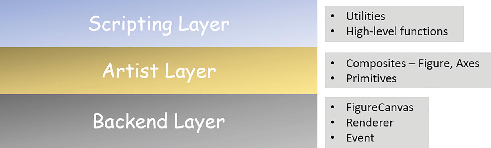
Matplotlib layers and core abstractions/objects
However, it is a great education for a data scientist to have deep knowledge about this layered architecture and follow the best practices that leverage the strength of a solid object-oriented design. In particular situations such as those involving subplots, this becomes prominent.
Two Approaches for Creating Panels with Subplots

Matplotlib subplots panel example
But why is the second approach better or more productive? Think about the cognitive load you might have to carry if it were 5 or 15 plots instead of 2 and the chances of bugs that could have been introduced writing code like plt.subplot(3, 1, 3) or plt.subplot(4, 4, 13). How would you keep track of all those parameters inside the plt.subplot() function? The second approach frees you from these considerations by allowing it to pass in a single number like 2 or 15 and repeat the plot statement that many times.
However, an even better approach is to put this code in a proper function that has a little more intelligence to handle any number of plots and that refactors the plotting statements using a loop.
A Better Approach with a Clever Function
Here, you can change the variable n to any value. Internally, the function will always calculate the appropriate number of rows with the logic in the code and set ncols = 3. Here, ax is a (multi-dimensional) list of Matplotlib Axes objects (https://matplotlib.org/stable/api/axes_api.html) and therefore can be indexed with axes[i] within a loop after you flatten the list with an axes = ax.ravel() statement.

Matplotlib panel function output with five plots

Matplotlib panel function output with 15 plots
It is the object-oriented style of programming pattern you embraced in your function definition that resulted in this scalable and efficient mechanism of generating any number of plots without worrying about potential bugs. This type of practice makes the codebase productive in the long run.
Set and Control Image Quality
Matplotlib interacts with the user’s graphical output system (web browser or stand-alone window) in a complex manner and optimizes the output image quality with a balanced set of internal settings. However, it is possible to tweak those settings as per the user’s preference to get the most optimum quality that they desire.
This becomes particularly important for using Matplotlib in the Jupyter notebook environment, which is an extremely common scenario. The quality of the default image, rendered in a Jupyter notebook web browser, may not be good enough for publication in a book or further processing. Data scientists often spend additional time and effort enhancing the quality of the visualizations they produce as part of the data science tasks. However, Matplotlib provides a simple and intuitive workaround to accomplish the same.
Setting DPI Directly in plt.figure()
In a Jupyter notebook, the default DPI value is quite low. Depending on your system settings, it is generally between 70 and 100. When you increase it, your figure also gets bigger, so you have to be mindful of not clipping the image in your browser window.
Setting DPI and Output Format for Saving Figures
When you choose JPEG as the output format, you can control a host of other settings related to the JPEG compression. However, PNG or PDF are better in terms of publication-worthy quality since they are lossless formats.
It depends on the intended usage, of course. For print, 150dpi is considered low-quality printing, even though 72dpi is considered the standard for the web (which is why it’s not easy printing quality images straight from the web). Low-resolution images will have blurring and pixelation (https://en.wikipedia.org/wiki/Pixilation) after printing. Medium-resolution images have between 200dpi - 300dpi. The industry standard for quality photographs and image is typically 300dpi.
Adjust Global Parameters

Matplotlib global rcParams change illustration
If you have decided on a set of image quality and styling settings, you can store them in a local config file and just read the values at the beginning of your Jupyter notebook or Python script while importing Matplotlib. That way, every image produced by that script or in that Jupyter session will have the same look and feel. The output of the code above should look something like Figure 3-13.
Did you notice that the axes.facecolor was set to a hex string #c3e2e6 in the code above? Matplotlib accepts regular color names like red, green, or blue, or hex strings in its various internal settings. You can simply use an online color picker tool (https://imagecolorpicker.com/) and copy-paste the hex code for better styling of your image.
Tricks with Seaborn
Seaborn is a Python library built on top of Matplotlib with a concentrated focus on statistical visualizations like boxplots, histograms, and regression plots. Naturally, for data scientists, it is a great tool to use in a typical exploratory data analysis (EDA) phase. However, using Seaborn with a couple of simple tricks can improve the productivity of your EDA tasks.
Use Sampled Data for Large Datasets
Pairwise plots (relating every variable in a dataset to another one)
Histograms
Boxplots
It might be tempting to generate all these plots for all the features and their pairwise combination (for the pair plot). However, depending on the amount of data and possible combination for the pairwise plot, the number of raw visual elements can be overwhelming for your system to handle.
One quick fix to this situation is to use random sample (a small fraction) of the dataset for generating all these plots. If the data is not too skewed, then by looking at a random sample (or a few of them), you should get a good feeling about the pattern and distributions from a typical EDA anyway.
Here you pass on only 100 samples from the original DataFrame to the plotting function. Note that to maintain readability and data structure integrity, you should not randomly sample 100 rows from the DataFrame but use a built-in function to return another DataFrame and pass that along to the plotting function.
Use pandas Correlation with Seaborn heatmap
This is a trick to quickly visualize the correlation strengths between multiple features of your dataset with just two lines of code. This kind of trick should be standard part of your efficient data science toolkit.

Using the pandas correlation function with a Seaborn heatmap to get the correlation visualization quickly for any dataset
Use Special Seaborn Methods to Reduce Work
Doing a linear regression and creating the plots of residuals with residplot
Counting the occurrence of categorical variables and plotting them using countplot
Using clustermap to create a hierarchical colored diagram from a matrix dataset
Summary
In this chapter, I started by describing how NumPy is faster than native Python code and enumerated its speed efficiency in simple scenarios. I talked about the pros and cons of converting Python objects like lists and tuples to NumPy arrays before doing numerical processing. Then, I discussed the importance of vectorizing operations as much as possible for efficient data science pipelines. I also discussed some of the reading utilities that NumPy offers and how they can make your code compact and productive.
Next, I delved into the efficient use of the pandas framework by discussing various methods to iterate over DataFrames and accessing or setting values. Usage of modern, optimized file storage formats like Parquet (in the context of Apache Arrow and column-oriented data storage) were discussed at length. Some miscellaneous ideas like chaining and cleaning up orphan DataFrame were talked about next.
Finally, I showed some tips and tricks to be used with popular visualization libraries Matplotlib and Seaborn. The object-oriented layered structure of Matplotlib was shown to be a strong foundation for building efficient data science code for plotting. I also demonstrated various methods of controlling image quality and plot settings in a global manner (i.e., for a Python or Jupyter session). Sampled data was discussed as an idea to control the explosion of plots that can happen with large datasets.
These kind of tips and tricks are developed over time based on data analysis, numerical computing, and exploratory data visualization needs that arise from handling real-life datasets in projects that need to be efficient and productive from time and computing resources points of view. As a regular practitioner of data science, you will also develop your own tricks and make your data analysis and modeling code efficient. The ideas in this chapter are just introductory guiding pointers to get you to think in that direction.