
Chapter 4
Data-Parallel Execution Model
Chapter Outline
4.1 Cuda Thread Organization
4.2 Mapping Threads to Multidimensional Data
4.3 Matrix-Matrix Multiplication—A More Complex Kernel
4.4 Synchronization and Transparent Scalability
4.5 Assigning Resources to Blocks
4.6 Querying Device Properties
4.7 Thread Scheduling and Latency Tolerance
4.8 Summary
4.9 Exercises
Fine-grained, data-parallel threads are the fundamental means of parallel execution in CUDA. As we explained in Chapter 3, launching a CUDA kernel creates a grid of threads that all execute the kernel function. That is, the kernel function specifies the C statements that are executed by each individual thread at runtime. Each thread uses a unique coordinate, or thread index, to identify the portion of the data structure to process. The thread index can be organized multidimensionally to facilitate access to multidimensional arrays. This chapter presents more details on the organization, resource assignment, synchronization, and scheduling of threads in a grid. A CUDA programmer who understands these details is well equipped to express and understand the parallelism in high-performance CUDA applications.
Built-In Variables
Many programming languages have built-in variables. These variables have special meaning and purpose. The values of these variables are often preinitialized by the runtime system. For example, in a CUDA kernel function, gridDim, blockDim, blockIdx, and threadIdx are all built-in variables. Their values are preinitialized by the CUDA runtime systems and can be referenced in the kernel function. The programmers should refrain from using these variables for any other purpose.
4.1 Cuda Thread Organization
Recall from Chapter 3 that all CUDA threads in a grid execute the same kernel function and they rely on coordinates to distinguish themselves from each other and to identify the appropriate portion of the data to process. These threads are organized into a two-level hierarchy: a grid consists of one or more blocks and each block in turn consists of one or more threads. All threads in a block share the same block index, which can be accessed as the blockIdx variable in a kernel. Each thread also has a thread index, which can be accessed as the threadIdx variable in a kernel. To a CUDA programmer, blockIdx and threadIdx appear as built-in, preinitialized variables that can be accessed within kernel functions (see “Built-in Variables” sidebar). When a thread executes a kernel function, references to the blockIdx and threadIdx variables return the coordinates of the thread. The execution configuration parameters in a kernel launch statement specify the dimensions of the grid and the dimensions of each block. These dimensions are available as predefined built-in variables gridDim and blockDim in kernel functions.
Hierarchical Organizations
Like CUDA threads, many real-world systems are organized hierarchically. The U.S. telephone system is a good example. At the top level, the telephone system consists of “areas,” each of which corresponds to a geographical area. All telephone lines within the same area have the same three-digit area code. A telephone area is typically larger than a city. For example, many counties and cities of central Illinois are within the same telephone area and share the same area code 217. Within an area, each phone line has a seven-digit local phone number, which allows each area to have a maximum of about 10 million numbers. One can think of each phone line as a CUDA thread, the area code as the CUDA blockIdx, and the seven-digital local number as the CUDA threadIdx. This hierarchical organization allows the system to have a very large number of phone lines while preserving “locality” for calling the same area. That is, when dialing a phone line in the same area, a caller only needs to dial the local number. As long as we make most of our calls within the local area, we do not need to dial the area code. If we occasionally need to call a phone line in another area, we dial 1 and the area code, followed by the local number (this is the reason why no local number in any area should start with a 1). The hierarchical organization of CUDA threads also offers a form of locality. We will study this locality soon.
In general, a grid is a 3D array of blocks1 and each block is a 3D array of threads. The programmer can choose to use fewer dimensions by setting the unused dimensions to 1. The exact organization of a grid is determined by the execution configuration parameters (within <<< and >>>) of the kernel launch statement. The first execution configuration parameter specifies the dimensions of the grid in number of blocks. The second specifies the dimensions of each block in number of threads. Each such parameter is of dim3 type, which is a C struct with three unsigned integer fields, x, y, and z. These three fields correspond to the three dimensions.
For 1D or 2D grids and blocks, the unused dimension fields should be set to 1 for clarity. For example, the following host code can be used to launch the vecAddkernel() kernel function and generate a 1D grid that consists of 128 blocks, each of which consists of 32 threads. The total number of threads in the grid is 128×32=4,096.
dim3 dimBlock(128, 1, 1);
dim3 dimGrid(32, 1, 1);
vecAddKernel<<<dimGrid, dimBlock>>>(…);
Note that dimBlock and dimGrid are host code variables defined by the programmer. These variables can have names as long as they are of dim3 type and the kernel launch uses the appropriate names. For example, the following statements accomplish the same as the previous statements:
dim3 dog(128, 1, 1);
dim3 cat(32, 1, 1);
vecAddKernel<<<dog, cat>>>(…);
The grid and block dimensions can also be calculated from other variables. For example, the kernel launch in Figure 3.14 can be written as:
dim3 dimGrid(ceil(n/256.0), 1, 1);
dim3 dimBlock(256, 1, 1);
vecAddKernel<<<dimGrid, dimBlock>>>(…);
This allows the number of blocks to vary with the size of the vectors so that the grid will have enough threads to cover all vector elements. The value of variable n at kernel launch time will determine the dimension of the grid. If n is equal to 1,000, the grid will consist of four blocks. If n is equal to 4,000, the grid will have 16 blocks. In each case, there will be enough threads to cover all the vector elements. Once vecAddKernel() is launched, the grid and block dimensions will remain the same until the entire grid finishes execution.
For convenience, CUDA C provides a special shortcut for launching a kernel with 1D grids and blocks. Instead of using dim3 variables, one can use arithmetic expressions to specify the configuration of 1D grids and blocks. In this case, the CUDA C compiler simply takes the arithmetic expression as the x dimensions and assumes that the y and z dimensions are 1. This gives us the kernel launch statement shown in Figure 3.14:
vecAddKernel<<<ceil(n/256.0), 256>>>(…);
Within the kernel function, the x field of the predefined variables gridDim and blockDim are preinitialized according to the execution configuration parameters. For example, if n is equal to 4,000, references to gridDim.x and blockDim.x in the vectAddkernel kernel function will result in 16 and 256, respectively. Note that unlike the dim3 variables in the host code, the names of these variables within the kernel functions are part of the CUDA C specification and cannot be changed. That is, the gridDim and blockDim variables in the kernel function always reflect the dimensions of the grid and the blocks.
In CUDA C, the allowed values of gridDim.x, gridDim.y, and gridDim.z range from 1 to 65,536. All threads in a block share the same blockIdx.x, blockIdx.y, and blockIdx.z values. Among all blocks, the blockIdx.x value ranges between 0 and gridDim.x-1, the blockIdx.y value between 0 and gridDim.y-1, and the blockIdx.z value between 0 and gridDim.z-1. For the rest of this book, we will use the notation (x, y, z) for a 3D grid with x blocks in the x direction, y blocks in the y direction, and z blocks in the z direction.
We now turn our attention to the configuration of blocks. Blocks are organized into 3D arrays of threads. Two-dimensional blocks can be created by setting the z dimension to 1. One-dimensional blocks can be created by setting both the y and z dimensions to 1, as in the vectorAddkernel example. As we mentioned before, all blocks in a grid have the same dimensions. The number of threads in each dimension of a block is specified by the second execution configuration parameter at the kernel launch. Within the kernel, this configuration parameter can be accessed as the x, y, and z fields of the predefined variable blockDim.
The total size of a block is limited to 1,024 threads, with flexibility in distributing these elements into the three dimensions as long as the total number of threads does not exceed 1,024. For example, (512, 1, 1), (8, 16, 4), and (32, 16, 2) are all allowable blockDim values, but (32, 32, 2) is not allowable since the total number of threads would exceed 1,024.2
Note that the grid can have higher dimensionality than its blocks and vice versa. For example, Figure 4.1 shows a small toy example of a 2D (2, 2, 1) grid that consists of 3D (4, 2, 2) blocks. The grid can be generated with the following host code:
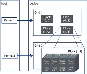
Figure 4.1 A multidimensional example of CUDA grid organization.
dim3 dimBlock(2, 2, 1);
dim3 dimGrid(4, 2, 2);
KernelFunction<<<dimGrid, dimBlock>>>(…);
The grid consists of four blocks organized into a 2×2 array. Each block in Figure 4.1 is labeled with (blockIdx.y, blockIdx.x). For example, block(1,0) has blockIdx.y=1 and blockIdx.x=0. Note that the ordering of the labels is such that the highest dimension comes first. This is reverse of the ordering used in the configuration parameters where the lowest dimension comes first. This reversed ordering for labeling threads works better when we illustrate the mapping of thread coordinates into data indexes in accessing multidimensional arrays.
Each threadIdx also consists of three fields: the x coordinate threadId.x, the y coordinate threadIdx.y, and the z coordinate threadIdx.z. Figure 4.1 illustrates the organization of threads within a block. In this example, each block is organized into 4×2×2 arrays of threads. Since all blocks within a grid have the same dimensions, we only need to show one of them. Figure 4.1 expands block(1,1) to show its 16 threads. For example, thread(1,0,2) has threadIdx.z=1, threadIdx.y=0, and threadIdx.x=2. Note that in this example, we have four blocks of 16 threads each, with a grand total of 64 threads in the grid. We use these small numbers to keep the illustration simple. Typical CUDA grids contain thousands to millions of threads.
4.2 Mapping Threads to Multidimensional Data
The choice of 1D, 2D, or 3D thread organizations is usually based on the nature of the data. For example, pictures are a 2D array of pixels. It is often convenient to use a 2D grid that consists of 2D blocks to process the pixels in a picture. Figure 4.2 shows such an arrangement for processing a 76×62 picture (76 pixels in the horizontal or x direction and 62 pixels in the vertical or y direction). Assume that we decided to use a 16×16 block, with 16 threads in the x direction and 16 threads in the y direction. We will need five blocks in the x direction and four blocks in the y direction, which results in 5×4=20 blocks as shown in Figure 4.2. The heavy lines mark the block boundaries. The shaded area depicts the threads that cover pixels. Note that we have four extra threads in the x direction and two extra threads in the y direction. That is, we will generate 80×64 threads to process 76×62 pixels. This is similar to the situation where a 1,000-element vector is processed by the 1D vecAddKernel in Figure 3.10 using four 256-thread blocks. Recall that an if statement is needed to prevent the extra 24 threads from taking effect. Analogously, we should expect that the picture processing kernel function will have if statements to test whether the thread indices threadIdx.x and threadIdx.y fall within the valid range of pixels.
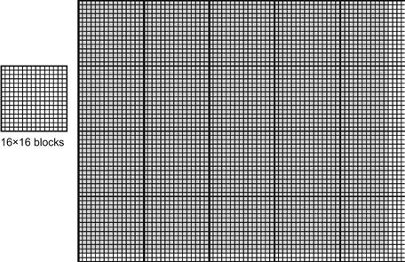
Figure 4.2 Using a 2D grid to process a picture.
Assume that the host code uses an integer variable n to track the number of pixels in the x direction, and another integer variable m to track the number of pixels in the y direction. We further assume that the input picture data has been copied to the device memory and can be accessed through a pointer variable d_Pin. The output picture has been allocated in the device memory and can be accessed through a pointer variable d_Pout. The following host code can be used to launch a 2D kernel to process the picture:
dim3 dimBlock(ceil(n/16.0), ceil(m/16.0), 1);
dim3 dimGrid(16, 16, 1);
pictureKernel<<<dimGrid, dimBlock>>>(d_Pin, d_Pout, n, m);
In this example, we assume for simplicity that the dimensions of the blocks are fixed at 16×16. The dimensions of the grid, on the other hand, depend on the dimensions of the picture. To process a 2,000×1,500 (3 M pixel) picture, we will generate 14,100 blocks, 150 in the x direction and 94 in the y direction. Within the kernel function, references to built-in variables gridDim.x, gridDim.y, blockDim.x, and blockDim.y will result in 150, 94, 16, and 16, respectively.
Before we show the kernel code, we need to first understand how C statements access elements of dynamically allocated multidimensional arrays. Ideally, we would like to access d_Pin as a 2D array where an element at row j and column i can be accessed as d_Pin[j][i]. However, the ANSI C standard based on which CUDA C was developed requires that the number of columns in d_Pin be known at compile time. Unfortunately, this information is not known at compiler time for dynamically allocated arrays. In fact, part of the reason why one uses dynamically allocated arrays is to allow the sizes and dimensions of these arrays to vary according to data size at runtime. Thus, the information on the number of columns in a dynamically allocated 2D array is not known at compile time by design. As a result, programmers need to explicitly linearize, or “flatten,” a dynamically allocated 2D array into an equivalent 1D array in the current CUDA C. Note that the newer C99 standard allows multidimensional syntax for dynamically allocated arrays. It is likely that future CUDA C versions may support multidimensional syntax for dynamically allocated arrays.
Memory Space
Memory space is a simplified view of how a processor accesses its memory in modern computers. A memory space is usually associated with each running application. The data to be processed by an application and instructions executed for the application are stored in locations in its memory space. Each location typically can accommodate a byte and has an address. Variables that require multiple bytes—4 bytes for float and 8 bytes for double—are stored in consecutive byte locations. The processor gives the starting address (address of the starting byte location) and the number of bytes needed when accessing a data value from the memory space.
The locations in a memory space are like phones in a telephone system where everyone has a unique phone number. Most modern computers have at least 4 GB-sized locations, where each G is 1,073,741,824 (230). All locations are labeled with an address that ranges from 0 to the largest number. Since there is only one address for every location, we say that the memory space has a “flat” organization. So, all multidimensional arrays are ultimately “flattened” into equivalent 1D arrays. While a C programmer can use a multidimensional syntax to access an element of a multidimensional array, the compiler translates these accesses into a base pointer that points to the beginning element of the array, along with an offset calculated from these multidimensional indices.
In reality, all multidimensional arrays in C are linearized. This is due to the use of a “flat” memory space in modern computers (see “Memory Space” sidebar). In the case of statically allocated arrays, the compilers allow the programmers to use higher-dimensional indexing syntax such as d_Pin[j][i] to access their elements. Under the hood, the compiler linearizes them into an equivalent 1D array and translates the multidimensional indexing syntax into a 1D offset. In the case of dynamically allocated arrays, the current CUDA C compiler leaves the work of such translation to the programmers due to lack of dimensional information.
There are at least two ways one can linearize a 2D array. One is to place all elements of the same row into consecutive locations. The rows are then placed one after another into the memory space. This arrangement, called row-major layout, is illustrated in Figure 4.3. To increase the readability, we will use Mj,i to denote an M element at the j row and the i column. Mj,i is equivalent to the C expression M[j][i] but slightly more readable. Figure 4.3 shows an example where a 4×4 matrix M is linearized into a 16-element 1D array, with all elements of row 0 first, followed by the four elements of row 1, etc. Therefore, the 1D equivalent index for the M element in row j and column i is j×4+i. The j×4 term skips over all elements of the rows before row j. The i term then selects the right element within the section for row j. For example, the 1D index for M2,1 is 2×4+1=9. This is illustrated in Figure 4.3, where M9 is the 1D equivalent to M2,1. This is the way C compilers linearize 2D arrays.
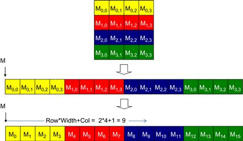
Figure 4.3 Row-major layout for a 2D C array. The result is an equivalent 1D array accessed by an index expression Row∗Width+Col for an element that is in the Rowth row and Colth column of an array of Width elements in each row.
Another way to linearize a 2D array is to place all elements of the same column into consecutive locations. The columns are then placed one after another into the memory space. This arrangement, called column-major layout, is used by FORTRAN compilers. Note that the column-major layout of a 2D array is equivalent to the row-major layout of its transposed form. We will not spend more time on this except mentioning that readers whose primary previous programming experience was with FORTRAN should be aware that CUDA C uses row-major layout rather than column-major layout. Also, many C libraries that are designed to be used by FORTRAN programs use column-major layout to match the FORTRAN compiler layout. As a result, the manual pages for these libraries, such as Basic Linear Algebra Subprograms (see “Linear Algebra Functions” sidebar), usually tell the users to transpose the input arrays if they call these libraries from C programs.
We are now ready to study the source code of pictureKernel(), shown in Figure 4.4. Let’s assume that the kernel will scale every pixel value in the picture by a factor of 2.0. The kernel code is conceptually quite simple. There are a total of blockDim.x∗gridDim.x threads in the horizontal direction. As we learned in the vecAddKernel() example, the expression Col= blockIdx.x∗blockDim.x+threadIdx.x generates every integer value from 0 to blockDim.x∗gridDim.x–1. We know that gridDim.x∗blockDim.x is greater than or equal to n. We have at least as many threads as the number of pixels in the horizontal direction. Similarly, we also know that there are at least as many threads as the number of pixels in the vertical direction. Therefore, as long as we test and make sure only the threads with both Row and Col values are within range, that is (Col<n) && (Row<m), we will be able to cover every pixel in the picture. Since there are n pixels in a row, we can generate the 1D index for the pixel at row Row and column Col as Row∗n+Col. This 1D index is used to read from the d_Pin array and write the d_Pout array.
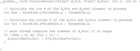
Figure 4.4 Source code of pictureKernel() showing a 2D thread mapping to a data pattern.
Figure 4.5 illustrates the execution of pictureKernel() when processing our 76×62 example. Assuming that we use 16×16 blocks, launching pictureKernel() generates 80×64 threads. The grid will have 20 blocks, 5 in the horizontal direction and 4 in the vertical direction. During the execution, the execution behavior of blocks will fill into one of four different cases, shown as four major areas in Figure 4.5.
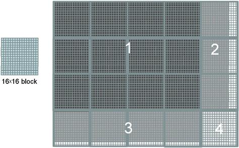
Figure 4.5 Covering a 76×62 picture with 16×16 blocks.
The first area, marked as 1 in Figure 4.5, consists of the threads that belong to the 12 blocks covering the majority of pixels in the picture. Both Col and Row values of these threads are within range; all these threads will pass the if statement test and process pixels in the dark-shaded area of the picture. That is, all 16×16=256 threads in each block will process pixels.
The second area, marked as 2 in Figure 4.5, contains the threads that belong to the 3 blocks in the medium-shaded area covering the upper-right pixels of the picture. Although the Row values of these threads are always within range, the Col values of some of them exceed the n value (76). This is because the number of threads in the horizontal direction is always a multiple of the blockDim.x value chosen by the programmer (16 in this case). The smallest multiple of 16 needed to cover 76 pixels is 80. As a result, 12 threads in each row will find their Col values within range and will process pixels. On the other hand, 4 threads in each row will find their Col values out of range, and thus fail the if statement condition. These threads will not process any pixels. Overall, 12×16=192 out of the 16×16=256 threads will process pixels.
The third area, marked as 3 in Figure 4.5, accounts for the 3 lower-left blocks covering the medium-shaded area of the picture. Although the Col values of these threads are always within range, the Row values of some of them exceed the m value (62). This is because the number of threads in the vertical direction is always multiples of the blockDim.y value chosen by the programmer (16 in this case). The smallest multiple of 16 to cover 62 is 64. As a result, 14 threads in each column will find their Row values within range and will process pixels. On the other hand, 2 threads in each column will fail the if statement of area 2, and will not process any pixels; 16×14=224 out of the 256 threads will process pixels.
The fourth area, marked as 4 in Figure 4.5, contains the threads that cover the lower-right light-shaded area of the picture. Similar to area 2, 4 threads in each of the top 14 rows will find their Col values out of range. Similar to area 3, the entire bottom two rows of this block will find their Row values out of range. So, only 14×12=168 of the 16×16=256 threads will be allowed to process threads.
We can easily extend our discussion of 2D arrays to 3D arrays by including another dimension when we linearize arrays. This is done by placing each “plane” of the array one after another. Assume that the programmer uses variables m and n to track the number of rows and columns in a 3D array. The programmer also needs to determine the values of blockDim.z and gridDim.z when launching a kernel. In the kernel, the array index will involve another global index:
int Plane = blockIdx.z∗blockDim.z + threadIdx.z
The linearized access to an array P will be in the form of P[Plane∗m∗n + Row ∗ n + Col]. One would of course need to test if all the three global indices—Plane, Row, and Col—fall within the valid range of the array.
Linear Algebra Functions
Linear algebra operations are widely used in science and engineering applications. According to the widely used basic linear algebra subprograms (BLAS), a de facto standard for publishing libraries that perform basic algebra operations, there are three levels of linear algebra functions. As the level increases, the amount of operations performed by the function increases. Level-1 functions perform vector operations of the form y=αx+y, where x and y are vectors and α is a scalar. Our vector addition example is a special case of a level-1 function with α=1. Level-2 functions perform matrix–vector operations of the form y=αAx+βy, where A is a matrix, x and y are vectors, and α and β are scalars. We will be studying a form of level-2 function in the context of sparse linear algebra. Level-3 functions perform matrix–matrix operations in the form of C=αAB+βC, where A, B, and C are matrices and α and β are scalars. Our matrix–matrix multiplication example is a special case of a level-3 function where α=1 and β=0. These BLAS functions are important because they are used as basic building blocks of higher-level algebraic functions such as linear system solvers and eigenvalue analysis. As we will discuss later, the performance of different implementations of BLAS functions can vary by orders of magnitude in both sequential and parallel computers.
4.3 Matrix-Matrix Multiplication—A More Complex Kernel
Up to this point, we have studied vecAddkernel() and pictureKernel() where each thread performs only one floating-point arithmetic operation on one array element. Readers should ask the obvious question: Do all CUDA threads perform only such a trivial amount of operation? The answer is no. Most real kernels have each thread to perform many more arithmetic operations and embody sophisticated control flows. These two simple kernels were selected for teaching the mapping of threads to data using threadIdx, blockIdx, blockDim, and gridDim variables. In particular, we introduce the following pattern of using global index values to ensure that every valid data element in a 2D array is covered by a unique thread:
Row = blockIdx.x∗blockDim.x+threadIdx.x
and
Col = blockIdx.y∗blockDim.y+threadIdx.y
We also used vecAddKernel() and pictureKernel() to introduce the phenomenon that the number of threads that we create is a multiple of the block dimension. As a result, we will likely end up with more threads than data elements. Not all threads will process elements of an array. We use an if statement to test if the global index values of a thread are within the valid range. Now that we understand the mapping of threads to data, we are in a position to understand kernels that perform more complex computation.
Matrix–matrix multiplication between an I×J matrix d_M and a J×K matrix d_N produces an I×K matrix d_P. Matrix–matrix multiplication is an important component of the BLAS standard (see “Linear Algebra Functions” sidebar). For simplicity, we will limit our discussion to square matrices, where I=J=K. We will use variable Width for I, J, and K.
When performing a matrix–matrix multiplication, each element of the product matrix d_P is an inner product of a row of d_M and a column of d_N. We will continue to use the convention where d_PRow,Col is the element at Row row and Col column. As shown in Figure 4.6, d_PRow, Col (the small square in d_P) is the inner product of the Row row of d_M (shown as the horizontal strip in d_M) and the Col column of d_N (shown as the vertical strip in d_N). The inner product between two vectors is the sum of products of corresponding elements. That is, d_PRow,Col=∑d_MRow,k ∗d_Nk,Col, for k = 0, 1, … Width-1. For example,
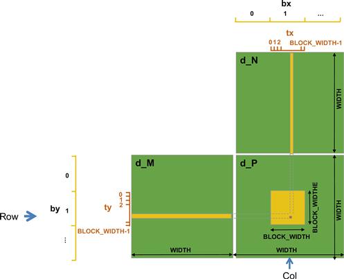
Figure 4.6 Matrix multiplication using multiple blocks by tiling d_P.
d_P1,5 = d_M1, 0∗d_N0,5 + d_M1,1∗d_N1,5 + d_M1,2∗ d_N2,5 +…. + d_M1,Width-1∗d_NWidth-1,5
We map threads to d_P elements with the same approach as what we used for pictureKernel(). That is, each thread is responsible for calculating one d_P element. The d_P element calculated by a thread is in row blockIdx.y∗blockDim.y+threadIdx.y and in column blockIdx.x∗blockDim.x+threadIdx.x. Figure 4.7 shows the source code of the kernel based on this thread-to-data mapping. Readers should immediately see the familiar pattern of calculating Row, Col, and the if statement testing if Row and Col are both within range. These statements are almost identical to their counterparts in pictureKernel(). The only significant difference is that we are assuming square matrices for the matrixMulKernel() so we replace both n and m with Width.
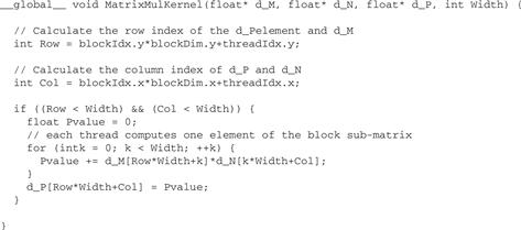
Figure 4.7 A simple matrix–matrix multiplication kernel using one thread to compute each d_P element.
With our thread-to-data mapping, we effectively divide d_P into square tiles, one of which is shown as a large square in Figure 4.6. Some dimension sizes may be better for a device and others may be better for another device. This is why, in real applications, programmers often want to keep the block dimensions as an easily adjustable value in the host code. A common practice is to declare a compile-time constant and use this constant in the host statements for setting the kernel launch configuration. We will refer to this compile-time constant as BLOCK_WIDTH. To set BLOCK_WIDTH to a value, say 16, we can use the following C statement in a header file or the beginning of a file where BLOCK_WIDTH is used:
#define BLOCK_WIDTH 16
Throughout the source code, instead of using a numerical value, the programmer can use the name BLOCK_WIDTH. Using a named compile-time constant allows the programmer to easily set BLOCK_WIDTH to a different value when compiling for a particular hardware. It also allows an automated tuning system to search for the best BLOCK_WIDTH value by iteratively setting it to different values, compile, and run for the hardware of interest. This type of process is often referred to as autotuning. In both cases, the source code can remain largely unchanged while changing the dimensions of the thread blocks.
Figure 4.8 shows the host code to be used to launch the matrixMulKernel(). Note that the configuration parameter dimGrid is set to ensure that for any combination of Width and BLOCK_WIDTH values, there are enough thread blocks in both x and y dimensions to calculate all d_P elements. Also, the name of the BLOCK_WIDTH constant rather than the actual value is used in initializing the fields of dimGrid and dimBlock. This allows the programmer to easily change the BLOCK_WIDTH value without modifying any of the other statements. Assume that we have a Width value of 1,000. That is, we need to do 1,000×1,000 matrix–matrix multiplication. For a BLOCK_WIDTH value of 16, we will generate 16×16 blocks. There will be 64×64 blocks in the grid to cover all d_P elements. By changing the #define statement in Figure 4.8 to
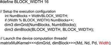
Figure 4.8 Host code for launching the matrixMulKernel() using a compile-time constant BLOCK_WIDTH to set up its configuration parameters.
#define BLOCK_WIDTH 32
we will generate 32×32 blocks. There will be 32×32 blocks in the grid. We can make this change to the kernel launch configuration without changing any of the statements that initialize dimGrid and dimBlock.
We now turn our attention to the work done by each thread. Recall that d_PRow, Col is the inner product of the Row row of d_M and the Col column of d_N. In Figure 4.7, we use a for loop to perform this inner product operation. Before we enter the loop, we initialize a local variable Pvalue to 0. Each iteration of the loop accesses an element in the Row row of d_M, an element in the Col column of d_N, multiplies the two elements together, and accumulates the product into Pvalue.
Let’s first focus on accessing the Row row of d_M within the for loop. Recall that d_M is linearized into an equivalent 1D array where the rows of d_M are placed one after another in the memory space, starting with the 0 row. Therefore, the beginning element of the 1 row is d_M[1∗Width] because we need to account for all elements of the 0 row. In general, the beginning element of the Row row is d_M[Row∗Width]. Since all elements of a row are placed in consecutive locations, the k element of the Row row is at d_M[Row∗Width+k]. This is what we used in Figure 4.7.
We now turn to accessing the Col column of d_N. As shown in Figure 4.3, the beginning element of the Col column is the Col element of the 0 row, which is d_N[Col]. Accessing each additional element in the Col column requires skipping over entire rows. This is because the next element of the same column is actually the same element in the next row. Therefore, the k element of the Col column is d_N[k∗Width+Col].
After the execution exits the for loop, all threads have their d_P element value in its Pvalue variable. It then uses the 1D equivalent index expression Row∗Width+Col to write its d_P element. Again, this index pattern is similar to that used in the pictureKernel(), with n replaced by Width.
We now use a small example to illustrate the execution of the matrix–matrix multiplication kernel. Figure 4.9 shows a 4×4 d_P with BLOCK_WIDTH = 2. The small sizes allow us to fit the entire example in one picture. The d_P matrix is now divided into four tiles and each block calculates one tile. (Whenever it is clear that we are discussing a device memory array, we will drop the d_ part of the name to improve readability. In Figure 4.10, we use P instead of d_P since it is clear that we are discussing a device memory array.) We do so by creating blocks that are 2×2 arrays of threads, with each thread calculating one P element. In the example, thread(0,0) of block(0,0) calculates P0,0, whereas thread(0,0) of block(1,0) calculates P2,0. It is easy to verify that one can identify the P element calculated by thread(0,0) of block(1,0) with the formula:
![]()
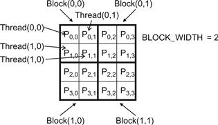
Figure 4.9 A small execution example of matrixMulKernel().
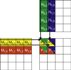
Figure 4.10 Matrix multiplication actions of one thread block. For readability, d_M, d_N, and d_P are shown as M, N, and P.
Readers should work through the index derivation for as many threads as it takes to become comfortable with the mapping.
Row and Col in the matrixMulKernel() identify the P element to be calculated by a thread. Row also identifies the row of M and Col identifies the column of N for input values for the thread. Figure 4.10 illustrates the multiplication actions in each thread block. For the small matrix multiplication, threads in block(0,0) produce four dot products. The Row and Col variables of thread(0,0) in block(0,0) are 0∗0+0= 0 and 0∗0+0=0. It maps to P0,0 and calculates the dot product of row 0 of M and column 0 of N.
We now walk through the execution of the for loop of Figure 4.7 for thread(0,0) in block(0,0). During the 0 iteration (k=0), Row∗Width+k = 0∗4+0 = 0 and k∗Width+Col = 0∗4+0 = 0. Therefore, the we are accessing d_M[0] and d_N[0], which according to Figure 4.3 are the 1D equivalent of d_M0,0 and d_N0,0. Note that these are indeed the 0 elements of row 0 of d_M and column 0 of d_N.
During the first iteration (k=1), Row∗Width+k = 0∗4+1 = 1 and k∗Width+Col = 1∗4+0 = 4. We are accessing d_M[1] and d_N[4], which according to Figure 4.3 are the 1D equivalent of d_M0,1 and d_N1,0. These are the first elements of row 0 of d_M and column 0 of d_N.
During the second iteration (k=2), Row∗Width+k = 0∗4+2 = 2 and k∗Width+Col = 8, which results in d_M[2] and d_N[8]. Therefore, the elements accessed are the 1D equivalent of d_M0,2 and d_N2,0.
Finally, during the third iteration (k=3), Row∗Width+k = 0∗4+3 and k∗Width+Col = 12, which results in d_M[3] and d_N[12], the 1D equivalent of dM0,3 and d_N3,0. We now have verified that the for loop performs the inner product between the 0 row of d_M and the 0 column of d_N. After the loop, the thread writes d_P[Row∗Width+Col], which is d_P[0]. This is the 1D equivalent of d_P0,0 so thread(0,0) in block(0,0) successfully calculated the inner product between the 0 row of d_M and the 0 column of d_N and deposited the result in d_P0,0.
We will leave it as an exercise for the reader to hand-execute and verify the for loop for other threads in block(0,0) or in other blocks.
Note that matrixMulKernel()can handle matrices of up to 16×65,535 elements in each dimension. In the situation where matrices larger than this limit are to be multiplied, one can divide up the P matrix into submatrices of which the size can be covered by a kernel. We can then either use the host code to iteratively launch kernels to complete the P matrix or have the kernel code of each thread to calculate more P elements.
4.4 Synchronization and Transparent Scalability
So far, we have discussed how to launch a kernel for execution by a grid of threads. We have also explained how one can map threads to parts of the data structure. However, we have not yet presented any means to coordinate the execution of multiple threads. We will now study a basic coordination mechanism. CUDA allows threads in the same block to coordinate their activities using a barrier synchronization function __syncthreads(). Note that “__” actually consists of two “_” characters. When a kernel function calls __syncthreads(), all threads in a block will be held at the calling location until every thread in the block reaches the location. This ensures that all threads in a block have completed a phase of their execution of the kernel before any of them can move on to the next phase. We will discuss an important use case of __syncthreads() in Chapter 5.
Barrier synchronization is a simple and popular method of coordinating parallel activities. In real life, we often use barrier synchronization to coordinate parallel activities of multiple persons. For example, assume that four friends go to a shopping mall in a car. They can all go to different stores to shop for their own clothes. This is a parallel activity and is much more efficient than if they all remain as a group and sequentially visit all the stores of interest. However, barrier synchronization is needed before they leave the mall. They have to wait until all four friends have returned to the car before they can leave—the ones who finish earlier need to wait for those who finish later. Without the barrier synchronization, one or more persons can be left in the mall when the car leaves, which can seriously damage their friendship!
Figure 4.11 illustrates the execution of barrier synchronization. There are N threads in the block. Time goes from left to right. Some of the threads reach the barrier synchronization statement early and some of them much later. The ones that reach the barrier early will wait for those that arrive late. When the latest one arrives at the barrier, everyone can continue their execution. With barrier synchronization, “No one is left behind.”

Figure 4.11 An example execution timing of barrier synchronization.
In CUDA, a __syncthreads() statement, if present, must be executed by all threads in a block. When a __syncthread() statement is placed in an if statement, either all threads in a block execute the path that includes the __syncthreads() or none of them does. For an if-then-else statement, if each path has a __syncthreads() statement, either all threads in a block execute the __syncthreads() on the then path or all of them execute the else path. The two __syncthreads() are different barrier synchronization points. If a thread in a block executes the then path and another executes the else path, they would be waiting at different barrier synchronization points. They would end up waiting for each other forever. It is the responsibility of the programmers to write their code so that these requirements are satisfied.
The ability to synchronize also imposes execution constraints on threads within a block. These threads should execute in close time proximity with each other to avoid excessively long waiting times. In fact, one needs to make sure that all threads involved in the barrier synchronization have access to the necessary resources to eventually arrive at the barrier. Otherwise, a thread that never arrived at the barrier synchronization point can cause everyone else to wait forever. CUDA runtime systems satisfy this constraint by assigning execution resources to all threads in a block as a unit. A block can begin execution only when the runtime system has secured all the resources needed for all threads in the block to complete execution. When a thread of a block is assigned to an execution resource, all other threads in the same block are also assigned to the same resource. This ensures the time proximity of all threads in a block and prevents excessive or indefinite waiting time during barrier synchronization.
This leads us to a major trade-off in the design of CUDA barrier synchronization. By not allowing threads in different blocks to perform barrier synchronization with each other, the CUDA runtime system can execute blocks in any order relative to each other since none of them need to wait for each other. This flexibility enables scalable implementations as shown in Figure 4.12, where time progresses from top to bottom. In a low-cost system with only a few execution resources, one can execute a small number of blocks at the same time; two blocks executing at a time is shown on the left side of Figure 4.12. In a high-end implementation with more execution resources, one can execute a large number of blocks at the same time; four blocks executing at a time is shown on the right side of Figure 4.12.
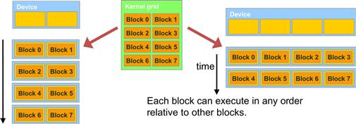
Figure 4.12 Lack of synchronization constraints between blocks enables transparent scalability for CUDA programs.
The ability to execute the same application code at a wide range of speeds allows the production of a wide range of implementations according to the cost, power, and performance requirements of particular market segments. For example, a mobile processor may execute an application slowly but at extremely low power consumption, and a desktop processor may execute the same application at a higher speed while consuming more power. Both execute exactly the same application program with no change to the code. The ability to execute the same application code on hardware with a different number of execution resources is referred to as transparent scalability, which reduces the burden on application developers and improves the usability of applications.
4.5 Assigning Resources to Blocks
Once a kernel is launched, the CUDA runtime system generates the corresponding grid of threads. As we discussed in the previous section, these threads are assigned to execution resources on a block-by-block basis. In the current generation of hardware, the execution resources are organized into streaming multiprocessors (SMs). Figure 4.13 illustrates that multiple thread blocks can be assigned to each SM. Each device has a limit on the number of blocks that can be assigned to each SM. For example, a CUDA device may allow up to eight blocks to be assigned to each SM. In situations where there is an insufficient amount of any one or more types of resources needed for the simultaneous execution of eight blocks, the CUDA runtime automatically reduces the number of blocks assigned to each SM until their combined resource usage falls under the limit. With a limited numbers of SMs and a limited number of blocks that can be assigned to each SM, there is a limit on the number of blocks that can be actively executing in a CUDA device. Most grids contain many more blocks than this number. The runtime system maintains a list of blocks that need to execute and assigns new blocks to SMs as they complete executing the blocks previously assigned to them.
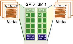
Figure 4.13 Thread block assignment to SMs.
Figure 4.13 shows an example in which three thread blocks are assigned to each SM. One of the SM resource limitations is the number of threads that can be simultaneously tracked and scheduled. It takes hardware resources for SMs to maintain the thread and block indices and track their execution status. In more recent CUDA device designs, up to 1,536 threads can be assigned to each SM. This could be in the form of 6 blocks of 256 threads each, 3 blocks of 512 threads each, etc. If the device only allows up to 8 blocks in an SM, it should be obvious that 12 blocks of 128 threads each is not a viable option. If a CUDA device has 30 SMs and each SM can accommodate up to1,536 threads, the device can have up to 46,080 threads simultaneously residing in the CUDA device for execution.
4.6 Querying Device Properties
Our discussions on assigning execution resources to blocks raise an important question: How do we find out the amount of resources available? When a CUDA application executes on a system, how can it find out the number of SMs in a device and the number of threads that can be assigned to each SM? Obviously, there are also other resources that we have not discussed so far but can be relevant to the execution of a CUDA application. In general, many modern applications are designed to execute on a wide variety of hardware systems. There is often a need for the application to query the available resources and capabilities of the underlying hardware to take advantage of the more capable systems while compensating for the less capable systems.
Resource and Capability Queries
In everyday life, we often query the resources and capabilities. For example, when we make a hotel reservation, we can check the amenities that come with a hotel room. If the room comes with a hair dryer, we do not need to bring one. Most American hotel rooms come with hair dryers while many hotels in other regions do not have them.
Some Asian and European hotels provide toothpastes and even toothbrushes while most American hotels do not. Many American hotels provide both shampoo and conditioner while hotels in other continents often only provide shampoo.
If the room comes with a microwave oven and a refrigerator, we can take the leftover from dinner and expect to eat it the second day. If the hotel has a pool, we can bring swim suits and take a dip after business meetings. If the hotel does not have a pool but has an exercise room, we can bring running shoes and exercise clothes. Some high-end Asian hotels even provide exercise clothing!
These hotel amenities are part of the properties, or resources and capabilities, of the hotels. Veteran travelers check these properties at hotel web sites, choose the hotels that better match their needs, and pack more efficiently and effectively using the information.
In CUDA C, there is a built-in mechanism for host code to query the properties of the devices available in the system. The CUDA runtime system has an API function cudaGetDeviceCount() that returns the number of available CUDA devices in the system. The host code can find out the number of available CUDA devices using the following statements:
int dev_count;
cudaGetDeviceCount( &dev_count);
While it may not be obvious, a modern PC system can easily have two or more CUDA devices. This is because many PC systems come with one or more “integrated” GPUs. These GPUs are the default graphics units and provide rudimentary capabilities and hardware resources to perform minimal graphics functionalities for modern window-based user interfaces. Most CUDA applications will not perform very well on these integrated devices. This would be a reason for the host code to iterate through all the available devices, query their resources and capabilities, and choose the ones that have enough resources to execute the application with satisfactory performance.
The CUDA runtime system numbers all the available devices in the system from 0 to dev_count-1. It provides an API function cudaGetDeviceProperties() that returns the properties of the device of which the number is given as an argument. For example, we can use the following statements in the host code to iterate through the available devices and query their properties:
cudaDeviceProp dev_prop;
for (I = 0; i<dev_count; i++) {
cudaGetDeviceProperties( &dev_prop, i);
// decide if device has sufficient resources and capabilities
}
The built-in type cudaDeviceProp is a C structure with fields that represent the properties of a CUDA device. Readers are referred to the CUDA Programming Guide for all the fields of the type. We will discuss a few of these fields that are particularly relevant to the assignment of execution resources to threads. We assume that the properties are returned in the dev_prop variable of which the fields are set by the cudaGetDeviceProperties() function. If readers choose to name the variable differently, the appropriate variable name will obviously need to be substituted in the following discussion.
As the name suggests, the field dev_prop.maxThreadsPerBlock gives the maximal number of threads allowed in a block in the queried device. Some devices allow up to 1,024 threads in each block and other devices allow fewer. It is possible that future devices may even allow more than 1,024 threads per block. Therefore, it is a good idea to query the available devices and determine which ones will allow a sufficient number of threads in each block as far as the application is concerned.
The number of SMs in the device is given in dev_prop.multiProcessorCount. As we discussed earlier, some devices have only a small number of SMs (e.g., 2) and some have a much larger number of SMs (e.g., 30). If the application requires a large number of SMs to achieve satisfactory performance, it should definitely check this property of the prospective device. Furthermore, the clock frequency of the device is in dev_prop.clockRate. The combination of the clock rate and the number of SMs gives a good indication of the hardware execution capacity of the device.
The host code can find the maximal number of threads allowed along each dimension of a block in dev_prop.maxThreadsDim[0] (for the x dimension), dev_prop.maxThreadsDim[1] (for the y dimension), and dev_prop.maxThreadsDim[2] (for the z dimension). An example use of this information is for an automated tuning system to set the range of block dimensions when evaluating the best performing block dimensions for the underlying hardware. Similarly, it can find the maximal number of blocks allowed along each dimension of a grid in dev_prop.maxGridSize[0] (for the x dimension), dev_prop.maxGridSize[1] (for the y dimension), and dev_prop.maxGridSize[2] (for the z dimension). A typical use of this information is to determine whether a grid can have enough threads to handle the entire data set or if some kind of iteration is needed.
There are many more fields in the cudaDeviceProp structure type. We will discuss them as we introduce the concepts and features that they are designed to reflect.
4.7 Thread Scheduling and Latency Tolerance
Thread scheduling is strictly an implementation concept and thus must be discussed in the context of specific hardware implementations. In most implementations to date, once a block is assigned to a SM, it is further divided into 32-thread units called warps. The size of warps is implementation-specific. In fact, warps are not part of the CUDA specification. However, knowledge of warps can be helpful in understanding and optimizing the performance of CUDA applications on particular generations of CUDA devices. The size of warps is a property of a CUDA device, which is in the dev_prop.warpSize field of the device query variable (dev_prop in this case).
The warp is the unit of thread scheduling in SMs. Figure 4.14 shows the division of blocks into warps in an implementation. Each warp consists of 32 threads of consecutive threadIdx values: threads 0–31 form the first warp, 32–63 the second warp, and so on. In this example, there are three blocks—block 1, block 2, and block 3, all assigned to an SM. Each of the three blocks is further divided into warps for scheduling purposes.
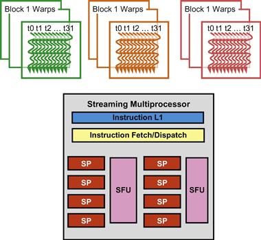
Figure 4.14 Blocks are partitioned into warps for thread scheduling.
We can calculate the number of warps that reside in an SM for a given block size and a given number of blocks assigned to each SM. For example, in Figure 4.14, if each block has 256 threads, we can determine that each block has 256÷32 or 8 warps. With three blocks in each SM, we have 8×3=24 warps in each SM.
An SM is designed to execute all threads in a warp following the single instruction, multiple data (SIMD) model. That is, at any instant in time, one instruction is fetched and executed for all threads in the warp. This is illustrated in Figure 4.14 with a single instruction fetch/dispatch shared among execution units in the SM. Note that these threads will apply the same instruction to different portions of the data. As a result, all threads in a warp will always have the same execution timing.
Figure 4.14 also shows a number of hardware streaming processors (SPs) that actually execute instructions. In general, there are fewer SPs than the number of threads assigned to each SM. That is, each SM has only enough hardware to execute instructions from a small subset of all threads assigned to the SM at any point in time. In earlier GPU design, each SM can execute only one instruction for a single warp at any given instant. In more recent designs, each SM can execute instructions for a small number of warps at any given point in time. In either case, the hardware can execute instructions for a small subset of all warps in the SM. A legitimate question is, why do we need to have so many warps in an SM if it can only execute a small subset of them at any instant? The answer is that this is how CUDA processors efficiently execute long-latency operations such as global memory accesses.
When an instruction executed by the threads in a warp needs to wait for the result of a previously initiated long-latency operation, the warp is not selected for execution. Another resident warp that is no longer waiting for results will be selected for execution. If more than one warp is ready for execution, a priority mechanism is used to select one for execution. This mechanism of filling the latency time of operations with work from other threads is often called latency tolerance or latency hiding (see “Latency Tolerance” sidebar).
Latency Tolerance
Latency tolerance is also needed in many everyday situations. For example, in post offices, each person trying to ship a package should ideally have filled out all the forms and labels before going to the service counter. However, as we have all experienced, many people wait for the service desk clerk to tell them which form to fill out and how to fill out the form.
When there is a long line in front of the service desk, it is important to maximize the productivity of the service clerks. Letting a person fill out the form in front of the clerk while everyone waits is not a good approach. The clerk should be helping the next customers who are waiting in line while the person fills out the form. These other customers are “ready to go” and should not be blocked by the customer who needs more time to fill out a form.
This is why a good clerk would politely ask the first customer to step aside to fill out the form while he or she can serve other customers. In most cases, the first customer will be served as soon as he or she finishes the form and the clerk finishes serving the current customer, instead of going to the end of the line.
We can think of these post office customers as warps and the clerk as a hardware execution unit. The customer who needs to fill out the form corresponds to a warp of which the continued execution is dependent on a long-latency operation.
Note that warp scheduling is also used for tolerating other types of operation latencies such as pipelined floating-point arithmetic and branch instructions. With enough warps around, the hardware will likely find a warp to execute at any point in time, thus making full use of the execution hardware in spite of these long-latency operations. The selection of ready warps for execution does not introduce any idle time into the execution timeline, which is referred to as zero-overhead thread scheduling. With warp scheduling, the long waiting time of warp instructions is “hidden” by executing instructions from other warps. This ability to tolerate long operation latencies is the main reason why GPUs do not dedicate nearly as much chip area to cache memories and branch prediction mechanisms as CPUs. As a result, GPUs can dedicate more of its chip area to floating-point execution resources.
We are now ready to do a simple exercise.3 Assume that a CUDA device allows up to 8 blocks and 1,024 threads per SM, whichever becomes a limitation first. Furthermore, it allows up to 512 threads in each block. For matrix–matrix multiplication, should we use 8×8, 16×16, or 32×32 thread blocks? To answer the question, we can analyze the pros and cons of each choice. If we use 8×8 blocks, each block would have only 64 threads. We will need 1,024÷64=12 blocks to fully occupy an SM. However, since there is a limitation of up to 8 blocks in each SM, we will end up with only 64×8=512 threads in each SM. This means that the SM execution resources will likely be underutilized because there will be fewer warps to schedule around long-latency operations.
The 16×16 blocks give 256 threads per block. This means that each SM can take 1,024÷256=4 blocks. This is within the 8-block limitation. This is a good configuration since we will have full thread capacity in each SM and a maximal number of warps for scheduling around the long-latency operations. The 32×32 blocks would give 1,024 threads in each block, exceeding the limit of 512 threads per block for this device.
4.8 Summary
The kernel execution configuration defines the dimensions of a grid and its blocks. Unique coordinates in blockIdx and threadIdx variables allow threads of a grid to identify themselves and their domains of data. It is the programmer’s responsibility to use these variables in kernel functions so that the threads can properly identify the portion of the data to process. This model of programming compels the programmer to organize threads and their data into hierarchical and multidimensional organizations.
Once a grid is launched, its blocks are assigned to SMs in arbitrary order, resulting in transparent scalability of CUDA applications. The transparent scalability comes with a limitation: threads in different blocks cannot synchronize with each other. To allow a kernel to maintain transparent scalability, the simple way for threads in different blocks to synchronize with each other is to terminate the kernel and start a new kernel for the activities after the synchronization point.
Threads are assigned to SMs for execution on a block-by-block basis. Each CUDA device imposes a potentially different limitation on the amount of resources available in each SM. For example, each CUDA device has a limit on the number of thread blocks and the number of threads each of its SMs can accommodate, whichever becomes a limitation first. For each kernel, one or more of these resource limitations can become the limiting factor for the number of threads that simultaneously reside in a CUDA device.
Once a block is assigned to an SM, it is further partitioned into warps. All threads in a warp have identical execution timing. At any time, the SM executes instructions of only a small subset of its resident warps. This allows the other warps to wait for long-latency operations without slowing down the overall execution throughput of the massive number of execution units.
4.9 Exercises
4.1 If a CUDA device’s SM can take up to 1,536 threads and up to 4 thread blocks, which of the following block configurations would result in the most number of threads in the SM?
4.2 For a vector addition, assume that the vector length is 2,000, each thread calculates one output element, and the thread block size is 512 threads. How many threads will be in the grid?
4.3 For the previous question, how many warps do you expect to have divergence due to the boundary check on the vector length?
4.4 You need to write a kernel that operates on an image of size 400×900 pixels. You would like to assign one thread to each pixel. You would like your thread blocks to be square and to use the maximum number of threads per block possible on the device (your device has compute capability 3.0). How would you select the grid dimensions and block dimensions of your kernel?
4.5 For the previous question, how many idle threads do you expect to have?
4.6 Consider a hypothetical block with 8 threads executing a section of code before reaching a barrier. The threads require the following amount of time (in microseconds) to execute the sections: 2.0, 2.3, 3.0, 2.8, 2.4, 1.9, 2.6, 2.9, and spend the rest of their time waiting for the barrier. What percentage of the threads’ summed-up execution times is spent waiting for the barrier?
4.7 Indicate which of the following assignments per multiprocessor is possible. In the case where it is not possible, indicate the limiting factor(s).
a. 8 blocks with 128 threads each on a device with compute capability 1.0
b. 8 blocks with 128 threads each on a device with compute capability 1.2
c. 8 blocks with 128 threads each on a device with compute capability 3.0
d. 16 blocks with 64 threads each on a device with compute capability 1.0
e. 16 blocks with 64 threads each on a device with compute capability 1.2
f. 16 blocks with 64 threads each on a device with compute capability 3.0
4.8 A CUDA programmer says that if they launch a kernel with only 32 threads in each block, they can leave out the __syncthreads() instruction wherever barrier synchronization is needed. Do you think this is a good idea? Explain.
4.9 A student mentioned that he was able to multiply two 1,024×1,024 matrices using a tiled matrix multiplication code with 32×32 thread blocks. He is using a CUDA device that allows up to 512 threads per block and up to 8 blocks per SM. He further mentioned that each thread in a thread block calculates one element of the result matrix. What would be your reaction and why?
4.10 The following kernel is executed on a large matrix, which is tiled into submatrices. To manipulate tiles, a new CUDA programmer has written the following device kernel, which will transpose each tile in the matrix. The tiles are of size BLOCK_WIDTH by BLOCK_WIDTH, and each of the dimensions of matrix A is known to be a multiple of BLOCK_WIDTH. The kernel invocation and code are shown below. BLOCK_WIDTH is known at compile time, but could be set anywhere from 1 to 20.
dim3 blockDim(BLOCK_WIDTH,BLOCK_WIDTH);
dim3 gridDim(A_width/blockDim.x,A_height/blockDim.y);
BlockTranspose<<<gridDim, blockDim>>>(A, A_width, A_height);
__global__ void
BlockTranspose(float∗ A_elements, int A_width, int A_height)
{
__shared__ float blockA[BLOCK_WIDTH][BLOCK_WIDTH];
int baseIdx = blockIdx.x ∗ BLOCK_SIZE + threadIdx.x;
baseIdx+ = (blockIdx.y ∗ BLOCK_SIZE + threadIdx.y) ∗ A_width;
blockA[threadIdx.y][threadIdx.x] = A_elements[baseIdx];
A_elements[baseIdx] = blockA[threadIdx.x][threadIdx.y];
}
a. Out of the possible range of values for BLOCK_SIZE, for what values of BLOCK_SIZE will this kernel function correctly when executing on the device?
b. If the code does not execute correctly for all BLOCK_SIZE values, suggest a fix to the code to make it work for all BLOCK_SIZE values.
1Devices with capability level less than 2.0 support grids with up to 2D arrays of blocks.
2Devices with capability less than 2.0 allow blocks with up to 512 threads.
3Note that this is an oversimplified exercise. As we will explain in Chapter 5, the usage of other resources, such as registers and shared memory, must also be considered when determining the most appropriate block dimensions. This exercise highlights the interactions between the limit on the number of thread blocks and the limit on the number of threads that can be assigned to each SM.