
Chapter 17
CUDA FORTRAN
Chapter Outline
17.1 CUDA FORTRAN and CUDA C Differences
17.2 A First CUDA FORTRAN Program
17.3 Multidimensional Array in CUDA FORTRAN
17.4 Overloading Host/Device Routines With Generic Interfaces
17.5 Calling CUDA C Via Iso_C_Binding
17.6 Kernel Loop Directives and Reduction Operations
17.7 Dynamic Shared Memory
17.8 Asynchronous Data Transfers
17.9 Compilation and Profiling
17.10 Calling Thrust from CUDA FORTRAN
17.11 Exercises
This chapter gives an introduction to CUDA FORTRAN, the FORTRAN interface to the CUDA architecture. CUDA FORTRAN was developed in 2009 as a joint effort between the Portland Group (PGI) and NVIDIA. CUDA FORTRAN shares much in common with CUDA C, as it is based on the runtime API, however, there are some differences in how the CUDA concepts are expressed using FORTRAN 90 constructs. The first section of this chapter discusses some of the basic differences between CUDA FORTRAN and CUDA C at a high level, and subsequent sections use various examples to illustrate CUDA FORTRAN programming.
17.1 CUDA FORTRAN and CUDA C Differences
CUDA FORTRAN and CUDA C have much in common, as CUDA FORTRAN is based on the CUDA C runtime API. Just as CUDA C is C with a few language extensions, CUDA FORTRAN is FORTRAN with a similar set of language extensions. Before we jump into CUDA FORTRAN code, it is helpful to summarize some of differences between these two programming interfaces to the CUDA architecture.
FORTRAN is a strongly typed language, and this strong typing carries over into the CUDA FORTRAN implementation. Device data declared in CUDA FORTRAN host code is declared with the device variable attribute, unlike CUDA C where both host and device data are declared the same way. Differentiating host and device data when variables are declared can simplify several aspects of dealing with device data. Allocation of device data can occur where the variable is declared, for example
real, device :: a_d(N)
will allocate a_d to contain N elements on device 0. Device data can also be declared as allocatable, and allocated using the FORTRAN 90’s allocate statement:
real, device, allocatable :: a_d(:)
…
allocate(a_d(N))
where the FORTRAN allocate routine has been overloaded to allocate arrays on the current device in the same way cudaMalloc does in CUDA C. CUDA FORTRAN’s strong typing also affects how data transfers between the host and the device can be performed. While one can use the CudaMemcpy function to perform host-to-device and device-to-host blocking transfers, it is far easier to use assignment statements:
real :: a(N)
real, device :: a_d(N)
…
a_d = a
where the FORTRAN array assignment kicks off a cudaMemcpy behind the scenes. Transfer via assignment statements applies only to blocking or synchronous transfers; for asynchronous transfers one must use the cudaMemcpyAsync call.
CUDA FORTRAN makes use of other variable attributes besides the device attribute. The attributes shared, constant, pinned, and value also find frequent use in CUDA FORTRAN. Shared memory used in device code uses the shared variable attribute just as CUDA C uses the __shared__ qualifier. Constant memory must be declared in a FORTRAN module that contains the device code where it is used, and the module must be used in the host code where it is initialized. The initialization of constant data in the host code is done via an assignment statement rather than by function calls. Pinned host memory is declared using the pinned variable attribute, and must also be declared allocatable. Since FORTRAN passes data by reference by default and in CUDA we typically deal with separate memory spaces for the host and the device, host parameters passed to a kernel via the argument list must be declared in the kernel with the value variable attribute.
CUDA FORTRAN also uses the attributes(global) and attributes(device) function attributes in the same way CUDA C uses declaration specifiers __global__ and __device__ to declare kernels and device functions.
Within CUDA FORTRAN device code the predefined variables gridDim, blockDim, blockIdx, and threadIdx are available as they are in CUDA C. Following typical FORTRAN convention, the components of blockIdx and threadIdx have a unit, rather than 0, offset, so a typical index calculation would look like the following:
i = blockDim%x ∗ (blockIdx%x - 1) + threadIdx%x
This is in contrast to CUDA C’s:
i = blockDim.x∗blockIdx.x + threadIdx.x;
This rounds out the major differences in the expression of CUDA concepts between CUDA C and CUDA FORTRAN. The CUDA FORTRAN notation will become clearer as we go through several examples in the following sections.
17.2 A First CUDA FORTRAN Program
The SAXPY routine has been used several times to illustrate various aspects of CUDA programming, and we continue this tradition with our first CUDA FORTRAN example:
module mathOps
contains
attributes(global) subroutine saxpy(x, y, a)
real :: x(:), y(:)
real, value :: a
integer :: i, n
n = size(x)
i = blockDim%x ∗ (blockIdx%x - 1) + threadIdx%x
if (i <= n) y(i) = y(i) + a∗x(i)
end subroutine saxpy
end module mathOps
program testSaxpy
use cudafor
use mathOps
implicit none
integer, parameter :: N = 40000
real :: x(N), y(N), a
real, device :: x_d(N), y_d(N)
type(dim3) :: grid, tBlock
tBlock = dim3(256,1,1)
grid = dim3(ceiling(real(N)/tBlock%x),1,1)
x = 1.0; y = 2.0; a = 2.0
x_d = x
y_d = y
call saxpy<<<grid,tBlock>>>(x_d, y_d, a)
y = y_d
write(∗,∗) ’Max error: ’, maxval(abs(y-4.0))
end program testSaxpy
In this complete code the SAXPY kernel is defined in the FORTRAN module mathOps using the attributes(global) qualifier. The kernel has three arguments: the 1D arrays x and y, and the scalar value a. The size of the x and y arrays does not need to be passed as a kernel argument since x and y are declared as assumed-shape arrays allowing the FORTRAN size() intrinsic to be used. Because a is defined on the host and must be passed by value, the value variable attribute is required in a’s declaration in the kernel. The predefined blockDim, blockIdx, and threadIdx variables are used to calculate a global index i used to access elements of x and y. Once again note that blockIdx and threadIdx have a unit offset as opposed to CUDA C’s zero offset. After checking for inbound access, the SAXPY operation is performed.
The host code uses the cudafor module, which defines CUDA runtime API routines, constants, and types, such as the type(dim3) used to declare the execution configuration variables grid and tBlock. In the host code, both host arrays x and y are declared as well as their device counterparts, x_d and y_d, where the latter are declared with the device variable attribute. The thread block and grid are defined in the first executable lines of host code, where the ceiling function is used to launch enough blocks to process all array elements in the case that the size of the array is not evenly divisible by the number of threads in a thread block. After the host arrays x and y, as well as the parameter a, are initialized, the assignment statements x_d=x and y_d=y are used to transfer the data from the host to the device. The scalar a is not passed to the device in this manner, as it is passed by value as a kernel argument. Since the transfers by assignment statement are blocking transfers, we can call the SAXPY kernel after the transfers without any synchronization. The kernel invocation specifies the execution configuration in the triple chevrons placed between the kernel name and its argument list as is done in CUDA C. Also similar to CUDA C, integer expressions can be used between the triple chevrons in place of the type(dim3) variables. This is followed by a device-to-host transfer of the resultant array, which is then checked for correctness.
17.3 Multidimensional Array in CUDA FORTRAN
Multidimensional arrays are first-class citizens in FORTRAN, and the ease of dealing with multidimensional data in FORTRAN is extended to CUDA FORTRAN. We have already seen one aspect of this in array assignments used for transfers between the host and the device. The ease of programming kernel code is evident from the following CUDA FORTRAN implementation of matrix multiply:
module mathOps
integer, parameter :: TILE_WIDTH = 16
contains
attributes(global) subroutine matrixMul(Md, Nd, Pd)
implicit none
real, intent(in) :: Md(:,:), Nd(:,:)
real, intent(out) :: Pd(:,:)
real, shared :: Mds(TILE_WIDTH, TILE_WIDTH)
real, shared :: Nds(TILE_WIDTH, TILE_WIDTH)
integer :: i, j, k, m, tx, ty, width
real :: Pvalue
tx = threadIdx%x; ty = threadIdx%y
i = (blockIdx%x-1)∗TILE_WIDTH + tx
j = (blockIdx%y-1)∗TILE_WIDTH + ty
width = size(Md,2)
Pvalue = 0.0
do m = 1, width, TILE_WIDTH
Mds(tx,ty) = Md(i,m+ty-1)
call syncthreads()
do k = 1, TILE_WIDTH
Pvalue = Pvalue + Mds(tx,k)∗Nds(k,ty)
enddo
call syncthreads()
enddo
Pd(i,j) = Pvalue
end subroutine matrixMul
end module mathOps
program testMatrixMultiply
use cudafor
use mathOps
implicit none
integer, parameter :: m=4∗TILE_WIDTH, n=6∗TILE_WIDTH, k=2∗TILE_WIDTH
real :: a(m,k), b(k,n), c(m,n), c2(m,n)
real, device :: a_d(m,k), b_d(k,n), c_d(m,n)
type(dim3) :: grid, tBlock
call random_number(a); a_d = a
call random_number(b); b_d = b
tBlock = dim3(TILE_WIDTH, TILE_WIDTH, 1)
grid = dim3(m/TILE_WIDTH, n/TILE_WIDTH, 1)
call matrixMul<<<grid, tBlock>>>(a_d, b_d, c_d)
c = c_d
! test against FORTRAN 90 matmul intrinsic
c2 = matmul(a, b)
write(∗,∗) ’max error: ’, maxval(abs(c-c2))
end program testMatrixMultiply
The matrixMul kernel uses shared memory tiles Mds and Nds just as in the CUDA C code, however, passing in 2D arrays as kernel arguments allows for a more intuitive indexing on the global arrays Md and Nd when copying to shared memory.
17.4 Overloading Host/Device Routines With Generic Interfaces
In the preceding matrix multiplication, we used the FORTRAN 90 matmul intrinsic to check our results. Because of the distinction between host and device data in the host code, it is possible to build generic interfaces that overload routines to execute either on the host or on the device depending on whether the arguments are host or device data. To illustrate how this is done, we present a generic interface to the matrix multiplication example in the previous section:
module mathOps
integer, parameter :: TILE_WIDTH = 16
interface matrixMultiply
module procedure mmCPU, mmGPU
end interface matrixMultiply
contains
function mmCPU(a, b) result(c)
implicit none
real :: a(:,:), b(:,:), c(:,:)
c = matmul(a,b)
end function mmCPU
function mmGPU(a_d, b_d) result(c)
use cudafor
implicit none
real, device :: a_d(:,:), b_d(:,:)
real :: c(:,:)
real, device, allocatable :: c_d(:,:)
integer :: m, n
type(dim3) :: grid, tBlock
m = size(c,1); n = size(c,2)
allocate(c_d(m,n))
tBlock = dim3(TILE_WIDTH, TILE_WIDTH, 1)
grid = dim3(m/TILE_WIDTH, n/TILE_WIDTH, 1)
call matrixMul<<<grid, tBlock>>>(a_d, b_d, c_d)
c = c_d
deallocate(c_d)
end function mmGPU
attributes(global) subroutine matrixMul(Md, Nd, Pd)
implicit none
real, intent(in) :: Md(:,:), Nd(:,:)
real, intent(out) :: Pd(:,:)
real, shared :: Mds(TILE_WIDTH, TILE_WIDTH)
real, shared :: Nds(TILE_WIDTH, TILE_WIDTH)
integer :: i, j, k, m, tx, ty, width
real :: Pvalue
tx = threadIdx%x; ty = threadIdx%y
i = (blockIdx%x-1)∗TILE_WIDTH + tx
j = (blockIdx%y-1)∗TILE_WIDTH + ty
width = size(Md,2)
Pvalue = 0.0
do m = 1, width, TILE_WIDTH
Mds(tx,ty) = Md(i,m+ty-1)
Nds(tx,ty) = Nd(m+tx-1,j)
call syncthreads()
do k = 1, TILE_WIDTH
Pvalue = Pvalue + Mds(tx,k)∗Nds(k,ty)
enddo
call syncthreads()
enddo
Pd(i,j) = Pvalue
end subroutine matrixMul
end module mathOps
program testMatrixMultiply
use cudafor
use mathOps
implicit none
integer, parameter :: m=4∗TILE_WIDTH, n=6∗TILE_WIDTH, k=2∗TILE_WIDTH
real :: a(m,k), b(k,n), c(m,n), c2(m,n)
real, device :: a_d(m,k), b_d(k,n)
call random_number(a); a_d = a
call random_number(b); b_d = b
c = matrixMultiply(a_d, b_d)
c2 = matrixMultiply(a, b)
write(∗,∗) ’max error: ’, maxval(abs(c-c2))
end program testMatrixMultiply
The interface to matrixMultiply in this code is overloaded using two procedures defined in the module, mmCPU and mmGPU. mmCPU operates on host data and simply calls the FORTRAN 90 intrinsic matmul. mmGPU takes device data for the input matrices, and returns a host array with the result. (It could just have easily been defined to return a device array.) The device array used for the result in mmGPU, c_d, is a local array that is declared on the sixth line of mmGPU, and allocated on the tenth line of that routine. After this allocation, the locally defined execution configuration parameters are determined and the kernel is launched, which is followed by a device-to-host transfer and the de-allocation of c_d. The actual matrix multiple kernel is not modified from the previous section. In the host code, matrixMultiply is used to access both of these routines.
17.5 Calling CUDA C Via Iso_C_Binding
In the previous section we demonstrated how an interface can be used to allow a single call to perform operations on either the host or device depending on where the input data resides. An interface can also be used to call C or CUDA C functions from CUDA FORTRAN using the iso_c_binding module introduced in FORTRAN 2003. Such functions can either be CUDA C routines developed by the user or library routines. In our matrix multiplication code, for example, we might wish to call the CUBLAS version of SGEMM rather than our hand-coded version. This can be done in the following manner:
module cublas_m
interface cublasInit
integer function cublasInit() bind(C,name=’cublasInit’)
end function cublasInit
end interface
interface cublasSgemm
subroutine cublasSgemm(cta,ctb,m,n,k,alpha,A,lda,B,ldb,beta,c,ldc) &
bind(C,name=’cublasSgemm’)
use iso_c_binding
character(1,c_char), value :: cta, ctb
integer(c_int), value :: k, m, n, lda, ldb, ldc
real(c_float), value :: alpha, beta
real(c_float), device :: A(lda,∗), B(ldb,∗), C(ldc,∗)
end subroutine cublasSgemm
end interface cublasSgemm
end module cublas_m
program sgemmDevice
use cublas_m
use cudafor
implicit none
integer, parameter :: m = 100, n = 100, k = 100
real :: a(m,k), b(k,n), c(m,n), c2(m,n)
real, device :: a_d(m,k), b_d(k,n), c_d(m,n)
real, parameter :: alpha = 1.0, beta = 0.0
integer :: lda = m, ldb = k, ldc = m
integer :: istat
call random_number(a); a_d = a
call random_number(b); b_d = b
istat = cublasInit()
call cublasSgemm(’n’,’n’,m,n,k,alpha,a_d,lda,b_d,ldb,beta,c_d,ldc)
c = c_d
c2 = matmul(a,b)
write(∗,∗) ’max error =’, maxval(abs(c-c2))
end program sgemmDevice
Here the module cublas_m contains interfaces for the CUBLAS routines cublasInit and cublasSgemm, which are bound to C functions as dictated by the bind(C,name=’…’) clause. The iso_c_binding module is used in the cublasSgemm interface as this module contains the type kind parameters used in the declarations for the function arguments.
One could manually write these interfaces for all of the CUBLAS routines, but this has already been done in the cublas module provided with the PGI CUDA FORTRAN compiler. In the preceding code, one can simply remove the cublas_m module and change the use cublas_m to use cublas in the main program. The cublas module also contains generic interfaces to overload the standard BLAS functions to execute the CUBLAS versions when the array arguments are device arrays. So we can further change the preceding program to call sgemm rather than cublasSgemm. The complete program then becomes as follows:
program sgemmDevice
use cublas
use cudafor
implicit none
integer, parameter :: m = 100, n = 100, k = 100
real :: a(m,k), b(k,n), c(m,n), c2(m,n)
real, device :: a_d(m,k), b_d(k,n), c_d(m,n)
real, parameter :: alpha = 1.0, beta = 0.0
integer :: lda = m, ldb = k, ldc = m
integer :: istat
call random_number(a); a_d = a
call random_number(b); b_d = b
istat = cublasInit()
call sgemm(’n’,’n’,m,n,k,alpha,a_d,lda,b_d,ldb,beta,c_d,ldc)
c = c_d
c2 = matmul(a,b)
write(∗,∗) ’max error =’, maxval(abs(c-c2))
17.6 Kernel Loop Directives and Reduction Operations
There are many occasions when one wishes to perform simple operations on device data, such as scaling or normalization of a device array. For such operations, it can be cumbersome to write separate kernels, and fortunately CUDA FORTRAN provides kernel CUDA FORTRAN loop directives, or CUF kernels. CUF kernels essentially allow the programmer to inline simple kernels in host code. For example, our SAXPY code using CUF kernels becomes
program testSaxpy
use cudafor
implicit none
integer, parameter :: N = 40000
real :: x(N), y(N), a
real, device :: x_d(N), y_d(N)
integer :: i
x = 1.0; x_d = x
y = 2.0; y_d = y
a = 2.0
!$cuf kernel do <<<∗,∗>>>
do i = 1, N
y_d(i) = y_d(i) + a∗x_d(i)
end do
y = y_d
write(∗,∗) ’Max error: ’, maxval(abs(y-4.0))
end program testSaxpy
In this complete code, the module containing the saxpy kernel has been removed and in its place in the host code is the loop that contains device arrays. The directive !$cuf kernel do informs the compiler to generate a kernel for the operation in the following do loop. The execution configuration can be manually specified in the <<<…,…>>>, or asterisks can be used to have the compiler choose an execution, as is done in this case. CUF kernels can operate on nested loops, and can use nondefault streams.
One particular useful aspect of CUF kernels is their ability to perform reductions. When the left side of an expression in a CUF kernel loop is a host scalar variable, a reduction operation is performed on the device. This is useful because coding a well-performing reduction in CUDA is not a trivial matter. The calculation of the sum of the device array elements using compiler-generated CUF kernels looks like the following:
program testReduction
use cudafor
implicit none
integer, parameter :: N = 40000
real :: x(N), xsum
real, device :: x_d(N)
integer :: i
x = 1.0; x_d = x
xsum = 0.0
!$cuf kernel do <<<∗,∗>>>
do i = 1, N
xsum = xsum + x_d(i)
end do
write(∗,∗) ’Error: ’, abs(xsum - sum(x))
end program testReduction
17.7 Dynamic Shared Memory
In our matrix multiplication example we demonstrated how static shared memory is used, which is essentially analogous to how it is declared in CUDA C. For dynamic shared memory, there are several options in CUDA FORTRAN. If a single dynamic shared memory array is used, then once again the CUDA FORTRAN implementation parallels what is done in CUDA C:
attributes(global) subroutine dynamicReverse1(d)
real :: d(:)
integer :: t, tr
real, shared :: s(∗)
t = threadIdx%x
tr = size(d)-t+1
s(t) = d(t)
call syncthreads()
d(t) = s(tr)
end subroutine dynamicReverse1
where the shared memory array s, used to reverse elements of a single thread block array in this kernel, is declared with as an assumed-size array. The size of this dynamic shared memory array is determined from the number of bytes of dynamic shared memory specified in the third execution configuration parameter:
threadBlock = dim3(n,1,1)
grid = dim3 (1 ,1 ,1)
…
call dynamicReverse1<<<grid,threadBlock,4∗threadBlock%x>>>(d_d)
When multiple dynamic shared memory arrays are used in CUDA C, essentially one large block of memory is allocated and pointer arithmetic is used to determine offsets into this block for the various variables. In CUDA FORTRAN, automatic arrays are used:
attributes (global) subroutine dynamicReverse2(d, nSize)
real :: d(nSize)
integer, value :: nSize
integer :: t, tr
real, shared :: s(nSize)
t = threadIdx%x
tr = nSize-t+1
s(t) = d(t)
call syncthreads()
d(t) = s(tr)
end subroutine dynamicReverse2
Here nSize is not known at compile time, hence s is not a static shared memory array. Any in-scope variable, such as a variable declared in the module that contains this kernel, can be used to determine the size of the automatic shared memory arrays. Multiple dynamic shared memory arrays of different types can be specified in this fashion. The total amount of dynamic shared memory must still be specified in the third execution configuration parameter.
17.8 Asynchronous Data Transfers
Asynchronous data transfers are performed using the cudaMemcpy∗Async() API calls as is done in CUDA C, with a couple of differences that apply not only to these asynchronous data transfer API calls but also to the synchronous cudaMemcpy∗() variants. The first difference is that the size of the transfer specified in the third argument is in terms of the number of elements rather than the number of bytes, and the second is that the direction of transfer is an optional argument since the direction can be inferred from the types of the first two arguments.
As with CUDA C, for asynchronous transfers the host memory must be pinned, which is accomplished through the pinned variable attribute rather than through a specific allocation function. Pinned memory in CUDA FORTRAN must be allocatable, and can be allocated and de-allocated through the FORTRAN 90 allocate() and deallocate() statements.
To overlap kernel execution and data transfers, in addition to pinned host memory, the data transfer and kernel must use different, nondefault streams. Nondefault streams are required for this overlap because memory copy, memory set functions, and kernel calls that use the default stream begin only after all preceding calls on the device (in any stream) have completed, and no operation on the device (in any stream) commences until they are finished. The following is an example of overlapping kernel execution and data transfer:
real, allocatable, pinned :: a(:)
…
integer (kind=cuda_stream_kind) :: stream1, stream2
…
allocate(a(nElements))
istat = cudaStreamCreate(stream1)
istat = cudaStreamCreate(stream2)
istat = cudaMemcpyAsync(a_d , a, nElements, stream1)
call kernel <<<gridSize ,blockSize ,0, stream2 >>>(b_d)
In this example, two streams are created and used in the data transfer and kernel executions as specified in the last arguments of the cudaMemcpyAsync() call and the kernels execution configuration. We make use of two device arrays, a_d and b_d, and assign work on a_d to stream1 and b_d to stream2.
If the operations on a single data array in a kernel are independent, then data can be broken into chunks and transferred in multiple stages, multiple kernels launched to operate on each chunk as it arrives, and each chunk’s results transferred back to the host when the relevant kernel completes. The following code segments demonstrate two ways of breaking up data transfers and kernel work to hide transfer time:
! baseline case - sequential transfer and execute
a = 0
istat = cudaEventRecord(startEvent ,0)
a_d = a
call kernel <<<n/blockSize , blockSize >>>(a_d, 0)
a = a_d
istat = cudaEventRecord(stopEvent , 0)
! Setup for multiple stream processing
strSize = n / nStreams
strGridSize = strSize / blocksize
i = 1, nStreams
istat = cudaStreamCreate(stream(i))
enddo
! asynchronous version 1: loop over {copy, kernel, copy}
a = 0
istat = cudaEventRecord(startEvent ,0)
do i = 1, nStreams
offset = (i-1)∗ strSize
istat=cudaMemcpyAsync(a_d(offset+1), a(offset+1), strSize, stream(i))
call kernel <<<strGridSize, blockSize, 0, stream(i)>>>(a_d, offset)
istat=cudaMemcpyAsync(a(offset+1), a_d(offset+1), strSize, stream(i))
enddo
istat = cudaEventRecord(stopEvent , 0)
! asynchronous version 2:
! loop over copy, loop over kernel, loop over copy
a = 0
istat = cudaEventRecord(startEvent ,0)
do i = 1, nStreams
offset = (i-1)∗ strSize
istat=cudaMemcpyAsync(a_d(offset+1), a(offset+1), strSize, stream(i))
enddo
do i = 1, nStreams
offset = (i-1)∗ strSize
call kernel <<<strGridSize, blockSize, 0, stream(i)>>>(a_d, offset)
enddo
do i = 1, nStreams
offset = (i-1)∗ strSize
istat = cudaMemcpyAsync(a(offset+1), a_d(offset+1), strSize ,stream(i))
enddo
istat = cudaEventRecord(stopEvent , 0)
The asynchronous cases are similar to the sequential case, only that there are multiple data transfers and kernel launches that are distinguished by different streams and an offset corresponding to the particular stream. In this code, we limit the number of streams to four, although for large arrays there is no reason why a larger number of streams could not be used. Note that the same kernel is used in the sequential and asynchronous cases in the code, as an offset is sent to the kernel to accommodate the data in different streams. The difference between the two asynchronous versions is the order in which the copies and kernels are executed. The first version loops over each stream and for each stream issues a host-to-device copy, kernel, and device-to-host copy. The second version issues all host-to-device copies, then all kernel launches, and then all device-to-host copies. We also make use of a third approach, which is a variant of the second where a dummy event is recorded after each kernel launch:
do i = 1, nStreams
offset = (i-1)∗ strSize
call kernel <<<strGridSize, blockSize, 0, stream(i)>>>(a_d, offset)
! Add a dummy event
istat = cudaEventRecord(dummyEvent, stream(i))
enddo
At this point you may be asking why we have three versions of the asynchronous case. The reason is that these variants perform differently on different hardware. Running this code on the NVIDIA Tesla C1060 produces the following:
Device: Tesla C1060
Time for sequential transfer and execute (ms): 12.92381
Time for asynchronous V1 transfer and execute (ms): 13.63690
Time for asynchronous V2 transfer and execute (ms): 8.845888
Time for asynchronous V3 transfer and execute (ms): 8.998560
And on the NVIDIA Tesla C2050 we get the following:
Device: Tesla C2050
Time for sequential transfer and execute (ms): 9.984512
Time for asynchronous V1 transfer and execute (ms): 5.735584
Time for asynchronous V2 transfer and execute (ms): 7.597984
Time for asynchronous V3 transfer and execute (ms): 5.735424
To decipher these results we need to understand a bit more about how devices schedule and execute various tasks. CUDA devices contain engines for various tasks, and operations are queued up in these engines as they are issued. Dependencies between tasks in different engines are maintained, but within any engine all dependence is lost, as tasks in an engine’s queue are executed in the order they are issued by the host thread. For example, the C1060 has a single copy engine and a single kernel engine. For the preceding code, timelines for the execution on the device are schematically shown in Figure 17.1. In this schematic we have assumed that the time required for the host-to-device transfer, kernel execution, and device-to-host transfer are approximately the same, and in the code provided, a kernel was chosen to make these times comparable.
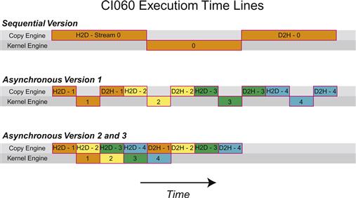
Figure 17.1 Data transfer and kernel execution timing for the sequential and asynchronous versions when there is only one copy engine.
For the sequential kernel, there is no overlap in any of the operations as one would expect. For the first asynchronous version of our code the order of execution in the copy engine is: H2D stream(1), D2H stream(1), H2D stream(2), D2H stream(2), and so forth. This is why we do not see any speedup when using the first asynchronous version on the C1060: tasks were issued to the copy engine in an order that precludes any overlap of kernel execution and data transfer. For versions two and three, however, where all the host-to-device transfers are issued before any of the device-to-host transfers, overlap is possible as indicated by the lower execution time. From our schematic, we would expect the execution of versions two and three to be 8/12 of the sequential version, or 8.7 ms, which is what is observed in the timing in the code.
On the C2050, two features interact to cause different behavior than that observed on the C1060. The C2050 has two copy engines, one for host-to-device transfers and another for device-to-host transfers, in addition to a single kernel engine. Having two copy engines explains why the first asynchronous version achieves good speedup on the C2050: the device-to-host transfer of data in stream(i) does not block the host-to-device transfer of data in stream(i+1) as it did on the C1060 because these two operations are in different engines on the C2050, which is schematically shown in Figure 17.2.
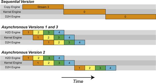
Figure 17.2 Data transfer and kernel execution timing for the sequential and asynchronous versions when there are two copy engines.
From the schematic we would expect the execution time to be cut in half relative to the sequential version, which is roughly what is observed in the timings in the code. This does not explain the performance degradation observed in the second asynchronous approach, however, which is related to the C2050’s support to concurrently run multiple kernels. When multiple kernels are issued back-to-back, the scheduler tries to enable concurrent execution of these kernels, and as a result delays a signal that normally occurs after each kernel completion (and is responsible for kicking off the device-to-host transfer) until all kernels complete. So, while there is overlap between host-to-device transfers and kernel execution in the second version of our asynchronous code, there is no overlap between kernel execution and device-to-host transfers. From Figure 17.2 one would expect an overall time for the second asynchronous version to be 9/12 of the time for the sequential version, or 7.5 ms, which is what we observe from the timings in the code. This situation can be rectified by recording a dummy CUDA event between each kernel, which will inhibit concurrent kernel execution but will enable overlap of data transfers and kernel execution, as is done in the third asynchronous version.
17.9 Compilation and Profiling
CUDA FORTRAN codes are compiled using PGI FORTRAN compiler. Files with the .cuf or .CUF extensions have CUDA FORTRAN enabled automatically, and the compiler option -Mcuda can be used when compiling a file with other extensions to enable CUDA FORTRAN. Compilation of CUDA FORTRAN code can be as simple as issuing the command
pgf90 saxpy.cuf
Behind the scenes, a multistep process takes place. The first step is a source-to-source compilation where CUDA C device code is generated by CUDA FORTRAN. From there, compilation is similar to compilation of CUDA C. The device code is compiled into the intermediate representation PTX, and the PTX code is then further compiled to an executable code for a particular compute capability. The host code is compiled using pgFORTRAN. The final executable contains the host binary, the device binary, and the PTX. The PTX is included so that a new device binary can be created when the executable is run on a card of different compute capability than originally compiled for.
Specifics of this compilation process can be controlled through options to -Mcuda. A specific compute capability can be targeted, for example, -Mcuda=cc20 generates executables for devices of compute capability 2.0. There is an emulation mode where device code is run on the host, specified by -Mcuda=emu. The specific version of the CUDA toolkit can be specified, for example, -Mcuda=cuda4.0 causes compilation with the 4.0 CUDA toolkit. CUDA has a set of fast, but less accurate, intrinsics for single-precision functions like sin() and cos(), which can be enabled by the -Mcuda=fastmath option. Use of these functions requires no change in the CUDA FORTRAN source code, as the intermediate CUDA C code will be generated with the corresponding __sinf() and __cosf() functions, respectively. For finer (selective) control, the latter versions are available when the cudadevice module is used in the device code. The option -Mucda=maxregcount:N can be used to limit the number of registers used per thread to N. And the option -Mcuda=ptxinfo prints information on memory usage in kernels. Multiple options to -Mcuda can be given in a comma-separated list, for example, -Mcuda=cc20,cuda4.0,ptxinfo.
Profiling CUDA FORTRAN codes can be performed using the command-line profiling facility used in CUDA C. Setting the environment variable COMPUTE_PROFILE to 1,
% export COMPUTE_PROFILE=1
and executing the code generates a file of profiling results, by default cuda_profile_0.log. For use of the command-line profiler see the documentation distributed with the CUDA toolkit.
17.10 Calling Thrust from CUDA FORTRAN
Previously, we demonstrated calling external CUDA C libraries from CUDA FORTRAN, in particular the CUBLAS library, using the iso_c_binding module. In this section we demonstrate how CUDA FORTRAN can interface with Thrust, the standard template library for the GPU discussed in Chapter 16. Relative to calling CUDA C functions, interfacing with Thrust requires the additional step of creating C pointers that access the Thrust device containers, such as in the following code segment:
// allocate device vector
thrust::device_vector d_vec(4);
// obtain raw pointer to device vector’s memory
int ∗ptr = thrust::raw_pointer_cast(&d_vec[0]);
The basic procedure to interface Thrust with CUDA FORTRAN is to create C wrapper functions that access Thrust’s functions through standard C pointers, and then use the iso_c_binding module to access these functions through a generic interface in CUDA FORTRAN. For an example, we use Thrust’s sort routine. The wrapper functions for the int, float, and double sort routines are as follows:
// Filename: csort.cu
// nvcc -c -arch sm_20 csort.cu
#include <thrust/device_vector.h>
#include <thrust/device_vector.h>
#include <thrust/sort.h>
extern "C" {
//Sort for integer arrays
void sort_int_wrapper( int ∗data, int N)
{
// Wrap raw pointer with a device_ptr
thrust::device_ptr <int> dev_ptr(data);
// Use device_ptr in Thrust sort algorithm
thrust::sort(dev_ptr, dev_ptr+N);
}
//Sort for float arrays
void sort_float_wrapper( float ∗data, int N)
{
thrust::device_ptr <float> dev_ptr(data);
thrust::sort(dev_ptr, dev_ptr+N);
}
//Sort for double arrays
void sort_double_wrapper( double ∗data, int N)
{
thrust::device_ptr <double> dev_ptr(data);
thrust::sort(dev_ptr, dev_ptr+N);
}
}
Compiling the code using
nvcc -c -arch sm_20 csort.cu
will generate an object file, csort.o, that we will use later on in the linking stage of the CUDA FORTRAN code.
With the C wrapper functions available, we can now write a FORTRAN module with a generic interface to Thust’s sort functionality:
module thrust
interface thrustsort
subroutine sort_int(input,N) bind(C,name="sort_int_wrapper")
use iso_c_binding
integer(c_int),device:: input(∗)
integer(c_int),value:: N
end subroutine sort_int
subroutine sort_float(input,N) bind(C,name="sort_float_wrapper")
use iso_c_binding
real(c_float),device:: input(∗)
integer(c_int),value:: N
end subroutine sort_float
subroutine sort_double(input,N) bind(C,name="sort_double_wrapper")
use iso_c_binding
real(c_double),device:: input(∗)
integer(c_int),value:: N
end subroutine sort_double
end interface thrustsort
With the C wrapper functions and the FORTRAN module written, we can now turn to the main FORTRAN code that generates and transfers the data to the device, calls the sort functions, and transfers the data back to the host:
program testsort
use thrust
! Declare two arrays, one on CPU (cpuData), one on GPU (gpuData)
real, allocatable :: cpuData(:)
real, allocatable, device :: gpuData(:)
integer:: N=10
! Allocate the arrays using standard allocate
allocate(cpuData(N),gpuData(N))
! Generate random numbers on the CPU
do i=1,N
cpuData(i)=random(i)
end do
cpuData(5)=100.
print ∗,"Before sorting", cpuData
! Copy the data to GPU with a simple assignment
gpuData=cpuData
! Call the Thrust sorting function. The generic interface will
! select the proper routine, in this case the one operating on floats
call thrustsort(gpuData,size(gpuData))
! Copy the data back to CPU with a simple assignment
cpuData=gpuData
print ∗,"After sorting", cpuData
! Deallocate the arrays using standard deallocate
allocate(cpuData(N),gpuData(N))
end program testsort
If we save the module in a file mod_thrust.cuf and the program in simplesort.cuf, we are ready to compile and execute:
$ pgf90 -Mcuda=cc20 -O3 -o simple_sort mod_thrust.cuf simple_sort.cuf csort.o
$ ./simple_sort
Before sorting 4.1630346E-02 0.9124327 0.7832350 0.6540373
100.0000 0.3956419 0.2664442 0.1372465
After sorting 8.0488138E-03 4.1630346E-02 0.1372465 0.2664442
0.3956419 0.6540373 0.7832350 0.8788511
0.9124327 100.0000
We can modify the main code to evaluate the performance using the CUDA event API as follows:
program timesort
use cudafor
use thrust
implicit none
real, allocatable :: cpuData(:)
real, allocatable, device :: gpuData(:)
integer:: i,N=100000000
! CUDA events for elapsing time
type (cudaEvent):: startEvent , stopEvent
real:: time, random
integer:: istat
! Create events
istat = cudaEventCreate(startEvent)
istat = cudaEventCreate(stopEvent)
! Allocate arrays
allocate(cpuData(N),gpuData(N))
do i=1,N
cpuData(i)=random(i)
end do
print ∗,"Sorting array of ",N, " single precision"
gpuData=cpuData
istat = cudaEventRecord ( startEvent , 0)
call thrustsort(gpuData,size(gpuData))
istat = cudaEventRecord ( stopEvent , 0)
istat = cudaEventSynchronize ( stopEvent )
istat = cudaEventElapsedTime ( time , startEvent , stopEvent )
cpuData=gpuData
print ∗," Sorted array in:",time," (ms)"
!Print the first five elements and the last five.
print ∗,"After sorting", cpuData(1:5),cpuData(N-4:N)
With the CUDA events, we are timing only the execution time of the sorting kernel. We can sort a vector of 100 M elements in 0.222 second on a Tesla M2050 with ECC on when the data is resident in GPU memory:
$ pgf90 -Mcuda=cc20 -O3 -o time_sort mod_thrust.cuf time_sort.cuf csort.o
$ ./time_sort
Sorting array of 100000000 single precision
Sorted array in: 222.1711 (ms)
After sorting 7.0585919E-09 1.0318221E-08 1.9398616E-08 3.1738640E-08
4.4078664E-08 0.9999999 0.9999999 1.000000 1.000000 1.000000