Chapter 3. Working with Financial Data
Clearly, data beats algorithms. Without comprehensive data, you tend to get non-comprehensive predictions.1
Rob Thomas
In algorithmic trading, one generally has to deal with four types of data as illustrated in Table 3-1. Although simplifying the real data world, distinguishing data along the pairs historical vs. real-time and structured vs. unstructured proves often useful in technical settings.
structured |
unstructured |
|
historical |
end-of-day closing prices |
financial news articles |
real-time |
bid/ask prices for FX |
posts on Twitter |
This book is mainly concerned with structured data (numerical, tabular data) of both historical and real-time types. This chapter in particular focuses on historical, structured data, like end-of-day closing values for the SAP SE stock traded at the Frankfurt Stock Exchange. However, this category also subsumes intraday data, like, for example, 1-minute-bar data for the Apple, Inc. stock traded at the NASDAQ stock exchange. The processing of real-time, structured data is covered in [Link to Come].
An algorithmic trading project typically starts with a trading idea or hypothesis which needs to be (back-)tested based on historical financial data. This is the context for this chapter, the plan for which is as follows. “Reading Financial Data From Different Sources” uses pandas to read data from different file- and web-based sources. “Working with Open Data Sources” introduces Quandl as a popular open data source platform. “Eikon Data API” introduces the Python wrapper for the Refinitiv Eikon Data API. Finally, “Storing Financial Data Efficiently” briefly shows how to store historical, structured data efficiently with pandas based on the HDF5 binary storage format.
The goal for this chapter is to have available financial data in a format with which the backtesting of trading ideas and hypotheses can be implemented effectively. The three major themes are the importing of data, the handling of the data and the storage of it. This and subsequent chapters assume a Python 3.8 installation with Python packages installed as explained in detail in Chapter 2. For the time being, it is not yet relevant on which infrastructure exactly this Python environment is provided. For more details on efficient input-output operations with Python, see Hilpisch (2018, ch. 9).
Reading Financial Data From Different Sources
This section makes heavy use of the capabilities of pandas, the popular data analysis package for Python (see pandas home page). pandas comprehensively supports the three main tasks this chapter is concerned with: reading data, handling data, and storing data. One of its strengths is the reading of data from different types of sources as the remainder of this section illustrates.
The Data Set
In this section, we work with a fairly small data set for the Apple, Inc. stock price (with symbol AAPL and Reuters Instrument Code or RIC AAPL.O) as retrieved from the Eikon Data API for April 2020.
Having stored such historical financial data in a CSV file on disk, pure Python can be used to read and print its content.
In[1]:fn='../data/AAPL.csv'In[2]:withopen(fn,'r')asf:for_inrange(5):(f.readline(),end='')Date,HIGH,CLOSE,LOW,OPEN,COUNT,VOLUME2020-04-01,248.72,240.91,239.13,246.5,460606.0,44054638.02020-04-02,245.15,244.93,236.9,240.34,380294.0,41483493.02020-04-03,245.7,241.41,238.9741,242.8,293699.0,32470017.02020-04-06,263.11,262.47,249.38,250.9,486681.0,50455071.0

Open the file on disk (adjust path and filename if necessary).

Sets up a
forloop with 5 iterations.
Prints the first 5 lines in the opened CSV file.
This approach allows for simple inspection of the data. One learns that there is a header line and that the single data points per row represent Date, OPEN, HIGH, LOW, CLOSE, COUNT and VOLUME, respectively. However, the data is not yet available in memory for further usage with Python.
Reading from a CSV File with Python
To work with data stored as a CSV file, the file needs to be parsed and the data needs to be stored in a Python data structure. Python has a built-in module called csv which supports the reading of data from a CSV file. The first approach yields a list object containing other list objects with the data from the file.
In[3]:importcsvIn[4]:csv_reader=csv.reader(open(fn,'r'))In[5]:data=list(csv_reader)In[6]:data[:5]Out[6]:[['Date','HIGH','CLOSE','LOW','OPEN','COUNT','VOLUME'],['2020-04-01','248.72','240.91','239.13','246.5','460606.0','44054638.0'],['2020-04-02','245.15','244.93','236.9','240.34','380294.0','41483493.0'],['2020-04-03','245.7','241.41','238.9741','242.8','293699.0','32470017.0'],['2020-04-06','263.11','262.47','249.38','250.9','486681.0','50455071.0']]
Imports the
csvmodule.Instantiates a
csv.readeriterator object.A
listcomprehension adding every single line from the CSV file as alistobject to the resultinglistobject.
Prints out the first five elements of the
listobject.
Working with such a nested list object — e.g. for the calculation of the average closing price — is possible in principle but not really efficient or intuitive. Using a csv.DictReader iterator object instead of the standard csv.reader object makes such tasks a bit more manageable. Every row of data in the CSV file (apart from the header row) is then imported as a dict object so that single values can be accessed via the respective key.
In[7]:csv_reader=csv.DictReader(open(fn,'r'))In[8]:data=list(csv_reader)In[9]:data[:3]Out[9]:[{'Date':'2020-04-01','HIGH':'248.72','CLOSE':'240.91','LOW':'239.13','OPEN':'246.5','COUNT':'460606.0','VOLUME':'44054638.0'},{'Date':'2020-04-02','HIGH':'245.15','CLOSE':'244.93','LOW':'236.9','OPEN':'240.34','COUNT':'380294.0','VOLUME':'41483493.0'},{'Date':'2020-04-03','HIGH':'245.7','CLOSE':'241.41','LOW':'238.9741','OPEN':'242.8','COUNT':'293699.0','VOLUME':'32470017.0'}]
Here, the
csv.DictReaderiterator object is instantiated which reads every data row into adictobject — given the information in the header row.
Based on the single dict objects, aggregations are now somewhat more easy to accomplish. However, one still cannot speak of a convenient way of calculating the mean of the Apple closing stock price when inspecting the respective Python code.
In[10]:sum([float(l['CLOSE'])forlindata])/len(data)Out[10]:272.38619047619045
First, a
listobject is generated via a list comprehension with all closing values; second, the sum is taken over all these values; third, the resulting sum is divided by the number of closing values.
This is one of the major reasons why pandas has gained such a popularity in the Python community. It makes the importing of data and the handling of, for example, financial time series data sets more convenient (and also often considerably faster) than pure Python.
Reading from a CSV File with pandas
From this point on, this section uses pandas to work with the Apple stock price data set. The major function used is read_csv() which allows for a number of customizations via different parameters (see the read_csv() API reference). read_csv() yields as a result of the data reading procedure a DataFrame object which is the central means of storing (tabular) data with pandas. The DataFrame class has many powerful methods that are particularly helpful in financial applications (refer to the DataFrame API reference).
In[11]:importpandasaspdIn[12]:data=pd.read_csv(fn,index_col=0,parse_dates=True)In[13]:data.info()<class'pandas.core.frame.DataFrame'>DatetimeIndex:21entries,2020-04-01to2020-04-30Datacolumns(total6columns):# Column Non-Null Count Dtype----------------------------0HIGH21non-nullfloat641CLOSE21non-nullfloat642LOW21non-nullfloat643OPEN21non-nullfloat644COUNT21non-nullfloat645VOLUME21non-nullfloat64dtypes:float64(6)memoryusage:1.1KBIn[14]:data.tail()Out[14]:HIGHCLOSELOWOPENCOUNTVOLUMEDate2020-04-24283.01282.97277.00277.20306176.031627183.02020-04-27284.54283.17279.95281.80300771.029271893.02020-04-28285.83278.58278.20285.08285384.028001187.02020-04-29289.67287.73283.89284.73324890.034320204.02020-04-30294.53293.80288.35289.96471129.045765968.0
The
pandaspackage is imported.This imports the data from the CSV file, indicated that the first column shall be treated as the index column and letting the entries in that column be interpreted as date-time information.
This method call prints out meta information regarding the resulting
DataFrameobject.The
data.tail()method prints out by default the five most recent data rows.
Calculating the mean of the Apple stock closing values now is only a single method call.
In[15]:data['CLOSE'].mean()Out[15]:272.38619047619056
Chapter 4 introduces more functionality of pandas for the handling of financial data. For details on working with pandas and the powerful DataFrame class also refer to the official pandas Documentation page and to the book McKinney (2017).
Tip
Although the Python standard library provides capabilities to read data from CSV files, pandas in general significantly simplifies and speeds up such operations. An additional benefit is that the data analysis capabilities of pandas are immediately available since read_csv() returns a DataFrame object.
Exporting to Excel and JSON
pandas also excels at exporting data stored in DataFrame objects when this data needs to be shared in a non-Python specific format. Apart from being able to export to CSV files, pandas allows, for example, also to do the export in the form of Excel spreadsheet files as well as JSON files which are both popular data exchange formats in the financial industry. Such an exporting procedure typically needs a single method call only.
In[16]:data.to_excel('data/aapl.xls','AAPL')In[17]:data.to_json('data/aapl.json')In[18]:ls-ndata/total24-rw-r--r--1501203067Aug2511:47aapl.json-rw-r--r--1501205632Aug2511:47aapl.xls
Exports the data to an Excel spreadsheet file on disk.
Exports the data to a JSON file on disk.
In particular when it comes to the interaction with Excel spreadsheet files, there are more elegant ways than just doing a data dump to a new file. xlwings, for example, is a powerful Python package allowing for an efficient and intelligent interaction between Python and Excel (visit the xlwings home page).
Reading from Excel and JSON
Now that the data is also available in the form of an Excel spreadsheet file and a JSON data file, pandas can read data from these sources as well. The approach is as straightforward as with CSV files.
In[19]:data_copy_1=pd.read_excel('data/aapl.xls','AAPL',index_col=0)In[20]:data_copy_1.head()Out[20]:HIGHCLOSELOWOPENCOUNTVOLUMEDate2020-04-01248.72240.91239.1300246.50460606440546382020-04-02245.15244.93236.9000240.34380294414834932020-04-03245.70241.41238.9741242.80293699324700172020-04-06263.11262.47249.3800250.90486681504550712020-04-07271.70259.43259.0000270.8046737550721831In[21]:data_copy_2=pd.read_json('data/aapl.json')In[22]:data_copy_2.head()Out[22]:HIGHCLOSELOWOPENCOUNTVOLUME2020-04-01248.72240.91239.1300246.50460606440546382020-04-02245.15244.93236.9000240.34380294414834932020-04-03245.70241.41238.9741242.80293699324700172020-04-06263.11262.47249.3800250.90486681504550712020-04-07271.70259.43259.0000270.8046737550721831In[23]:!rmdata/*
This reads the data from the Excel spreadsheet file to a new
DataFrameobject.The first five rows of the first in-memory copy of the data are printed.
This reads the data from the JSON file to yet another
DataFrameobject.This then prints the first five rows of the second in-memory copy of the data.
pandas proves useful for reading and writing financial data from and to different types of data files. Often, the reading might be tricky due to non-standard storage formats (like a “;” instead of a “,” as separator) but pandas generally provides the right set of parameter combinations to cope with such cases. Although all examples in this section use a small data set only, one can expect high performance input-output operations from pandas in the most important scenarios when the data sets are much larger.
Working with Open Data Sources
To a great extent, the attractiveness of the Python ecosystem stems from the fact that almost all packages available are open source and can be used for free. Financial analytics in general and algorithmic trading in particular, however, cannot live with open source software and algorithms alone — data plays a vital role as well, as the quote at the beginning of the chapter emphasizes. The previous section uses a small data set from a commercial data source. While there have been helpful open (financial) data sources available for some years (such as the ones provided by Yahoo! Finance or Google Finance), there are not too many left at the time of this writing in 2020. One of the more obvious reasons for this trend might be the ever-changing terms of data licensing agreements.
The one notable exception for the purposes of this book is Quandl (http://quandl.com), a platform that aggregates a large number of open as well as premium (= to-be-paid-for) data sources. The data is provided via a unified API for which a Python wrapper package is available.
The Python wrapper package for the Quandl data API (see the Python wrapper page on Quandl and the Github page of the package) is installed with conda through conda install quandl. The first example shows how to retrieve historical average prices for the BTC/USD exchange rate since the introduction of Bitcoin as a cryptocurrency. With Quandl, requests expect always a combination of the database and the specific data set desired. In the example, BCHAIN and MKPRU. Such information can generally be looked up on the Quandl platform. For the example, the relevant page on Quandl is BCHAIN/MKPRU.
By default, the quandl package returns a pandas DataFrame object. In the example, the Value column is also presented in annualized fashion, i.e. with year end values. Note that the number shown for 2020 is the last available value in the data set (from May 2020) and not necessarily the year end value.
While a large part of the data sets on the Quandl platform are free, some of the free data sets require an API key (such a key is required after a certain limit of free API calls too). Every user obtains such a key by signing up for a free Quandl account on the Quandl sign up page. Data requests requiring an API key expect the key to be provided as the parameter api_key. In the example, the API key (which is found on the account settings page) is stored as a string in the variable quandl_api_key. The concrete value for the key is read from a configuration file via the configparser module.
In[24]:importconfigparserconfig=configparser.ConfigParser()config.read('../pyalgo.cfg')Out[24]:['../pyalgo.cfg']In[25]:importquandlasqIn[26]:data=q.get('BCHAIN/MKPRU',api_key=config['quandl']['api_key'])In[27]:data.info()<class'pandas.core.frame.DataFrame'>DatetimeIndex:4254entries,2009-01-03to2020-08-26Datacolumns(total1columns):# Column Non-Null Count Dtype----------------------------0Value4254non-nullfloat64dtypes:float64(1)memoryusage:66.5KBIn[28]:data['Value'].resample('A').last()Out[28]:Date2009-12-310.0000002010-12-310.2999992011-12-314.9950002012-12-3113.5900002013-12-31731.0000002014-12-31317.4000002015-12-31428.0000002016-12-31952.1500002017-12-3113215.5740002018-12-313832.9216672019-12-317385.3600002020-12-3111763.930000Freq:A-DEC,Name:Value,dtype:float64
Imports the Python wrapper package for Quandl.
Reads historical data for the BTC/USD exchange rate.
Selects the
Valuecolumn, resamples it — from the originally daily values to yearly values — and defines the last available observation to be the relevant one.
Quandl also provides, for example, diverse data sets for single stocks, like end-of-day stock prices, stock fundamentals or data sets related to options traded on a certain stock.
In[29]:data=q.get('FSE/SAP_X',start_date='2018-1-1',end_date='2020-05-01',api_key=config['quandl']['api_key'])In[30]:data.info()<class'pandas.core.frame.DataFrame'>DatetimeIndex:579entries,2018-01-02to2020-04-30Datacolumns(total10columns):# Column Non-Null Count Dtype----------------------------0Open257non-nullfloat641High579non-nullfloat642Low579non-nullfloat643Close579non-nullfloat644Change0non-nullobject5TradedVolume533non-nullfloat646Turnover533non-nullfloat647LastPriceoftheDay0non-nullobject8DailyTradedUnits0non-nullobject9DailyTurnover0non-nullobjectdtypes:float64(6),object(4)memoryusage:49.8+KB
The API key can also be configured permanently with the Python wrapper via
q.ApiConfig.api_key='YOUR_API_KEY'
The Quandl platform also offers premium data sets for which a subscription or fee is required. Most of these data sets offer free samples. The example retrieves option implied volatilities for the Microsoft, Inc. stock. The free sample data set is quite large with more than 4,100 rows and many columns (only a subset is shown). The last line of code display the 30, 60 and 90 days implied volatility values for the five most recent days available.
In[31]:q.ApiConfig.api_key=config['quandl']['api_key']In[32]:vol=q.get('VOL/MSFT')In[33]:vol.iloc[:,:10].info()<class'pandas.core.frame.DataFrame'>DatetimeIndex:1006entries,2015-01-02to2018-12-31Datacolumns(total10columns):# Column Non-Null Count Dtype----------------------------0Hv101006non-nullfloat641Hv201006non-nullfloat642Hv301006non-nullfloat643Hv601006non-nullfloat644Hv901006non-nullfloat645Hv1201006non-nullfloat646Hv1501006non-nullfloat647Hv1801006non-nullfloat648Phv101006non-nullfloat649Phv201006non-nullfloat64dtypes:float64(10)memoryusage:86.5KBIn[34]:vol[['IvMean30','IvMean60','IvMean90']].tail()Out[34]:IvMean30IvMean60IvMean90Date2018-12-240.43100.41120.38292018-12-260.40590.38440.35872018-12-270.39180.38790.36182018-12-280.39400.37360.34822018-12-310.37600.35190.3310
This concludes the overview of the Python wrapper package quandl for the Quandl data API. The Quandl platform and service is growing rapidly and proves to be a valuable source for financial data in an algorithmic trading context.
Note
Open source software is a trend that started many years ago. It has lowered the barriers to entry in many areas and also in algorithmic trading. A new, reinforcing trend in this regard are open data sources. In some cases, such as with Quandl, they even provide high quality data sets. It cannot be expected that open data will completely replace professional data subscriptions any time soon, but they represent a valuable means to get started with algorithmic trading in a cost efficient manner.
Eikon Data API
Open data sources are a blessing for algorithmic traders wanting to get started in the space and wanting to be able to quickly test hypotheses and ideas based on real financial data sets. Sooner or later, however, open data sets will not suffice anymore to satisfy the requirements of more ambitious traders and professionals.
Refinitiv is one of the biggest financial data and news providers in the world. Its current desktop flagship product is Eikon which is the equivalent to the Terminal by Bloomberg, the major competitor in the data services field. Figure 3-1 shows a screen shot of Eikon in the browser-based version. It provides access to peta bytes of data via a single access point.
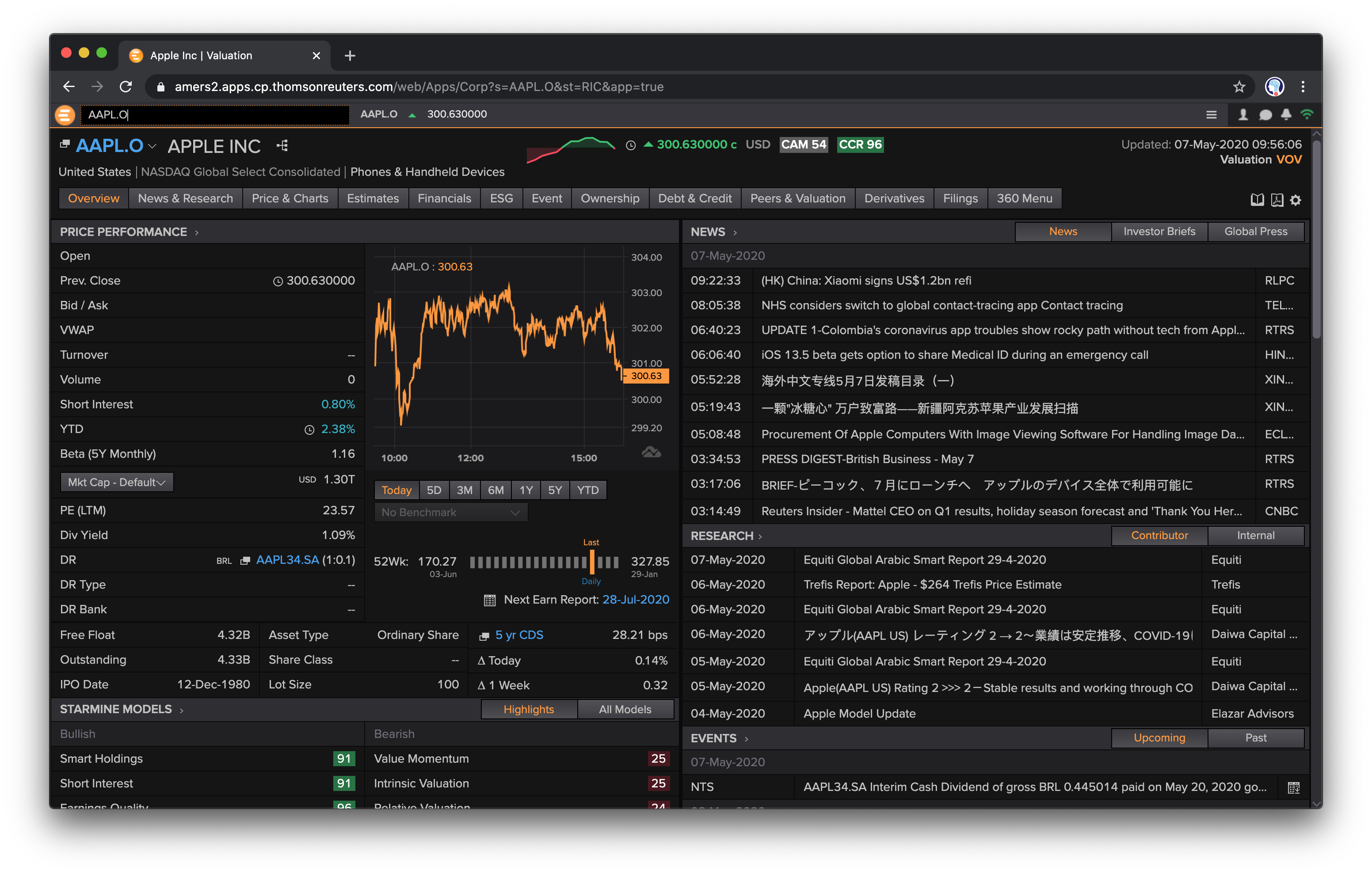
Figure 3-1. Browser version of Eikon terminal
Recently, Refinitiv have streamlined their API landscape and have released a Python wrapper package, called eikon, for the Eikon data API which is installed via pip install eikon. If you have a subscription to the Refinitiv Eikon data services, you can use the Python package to programmatically retrieve historical as well as streaming structured and unstructured data from the unified API. A technical prerequisite is that a local desktop application is running that provides a desktop API session. The latest such desktop application at the time of this writing is called Workspace (see Figure 3-2).

Figure 3-2. Workspace application with desktop API services
If you are an Eikon subscriber and have an account for the Developer Community pages, you find an overview of the Python Eikon Scripting Library under Quick Start.
In order to use the Eikon Data API, the Eikon app_key needs to be set. You get it via the App Key Generator (APPKEY`) application in either Eikon or Workspace.
In[35]:importeikonasekIn[36]:ek.set_app_key(config['eikon']['app_key'])In[37]:help(ek)Helponpackageeikon:NAMEeikon-# coding: utf-8PACKAGECONTENTSProfiledata_grideikonErrorjson_requestsnews_requeststreaming_session(package)symbologytime_seriestoolsSUBMODULEScachedesktop_sessionistream_callbackitemstreamsessionstreamstream_connectionstreamingpricestreamingprice_callbackstreamingpricesVERSION1.1.5FILE/Users/yves/Python/envs/py38/lib/python3.8/site-packages/eikon/__init__.py
Imports the
eikonpackage asek.Sets the
app_key.Shows the help text for the main module.
Retrieving Historical Structured Data
The retrieval of historical financial time series data is as straightforward as with the other wrappers used before.
In[39]:symbols=['AAPL.O','MSFT.O','GOOG.O']In[40]:data=ek.get_timeseries(symbols,start_date='2020-01-01',end_date='2020-05-01',interval='daily',fields=['*'])In[41]:data.keys()Out[41]:MultiIndex([('AAPL.O','HIGH'),('AAPL.O','CLOSE'),('AAPL.O','LOW'),('AAPL.O','OPEN'),('AAPL.O','COUNT'),('AAPL.O','VOLUME'),('MSFT.O','HIGH'),('MSFT.O','CLOSE'),('MSFT.O','LOW'),('MSFT.O','OPEN'),('MSFT.O','COUNT'),('MSFT.O','VOLUME'),('GOOG.O','HIGH'),('GOOG.O','CLOSE'),('GOOG.O','LOW'),('GOOG.O','OPEN'),('GOOG.O','COUNT'),('GOOG.O','VOLUME')],)In[42]:type(data['AAPL.O'])Out[42]:pandas.core.frame.DataFrameIn[43]:data['AAPL.O'].info()<class'pandas.core.frame.DataFrame'>DatetimeIndex:84entries,2020-01-02to2020-05-01Datacolumns(total6columns):# Column Non-Null Count Dtype----------------------------0HIGH84non-nullfloat641CLOSE84non-nullfloat642LOW84non-nullfloat643OPEN84non-nullfloat644COUNT84non-nullInt645VOLUME84non-nullInt64dtypes:Int64(2),float64(4)memoryusage:4.8KBIn[44]:data['AAPL.O'].tail()Out[44]:HIGHCLOSELOWOPENCOUNTVOLUMEDate2020-04-27284.54283.17279.95281.80300771292718932020-04-28285.83278.58278.20285.08285384280011872020-04-29289.67287.73283.89284.73324890343202042020-04-30294.53293.80288.35289.96471129457659682020-05-01299.00289.07285.85286.2555831960154175
Defines a few symbols as a
listobject.The central line of code that retrieves data for the first symbol …
… for the given start date and …
… the given end date.

The time interval is here chosen to be
daily.
All fields are requested.

The function
get_timeseries()returns a multi-indexDataFrameobject.
The values corresponding to each level are regular
DataFrameobjects.
This provides an overview of the data stored in the
DataFrameobject.
The final five rows of data are shown.
The beauty of working with a professional data service API becomes evident when one wishes to work with multiple symbols and in particular with a different granularity of the financial data, i.e. other time intervals.
In[45]:%%timedata=ek.get_timeseries(symbols,start_date='2020-08-14',end_date='2020-08-15',interval='minute',fields='*')CPUtimes:user58.2ms,sys:3.16ms,total:61.4msWalltime:2.02sIn[46]:(data['GOOG.O'].loc['2020-08-14 16:00:00':'2020-08-14 16:04:00'])HIGHLOWOPENCLOSECOUNTVOLUMEDate2020-08-1416:00:001510.74391509.2201509.9401510.52394813622020-08-1416:01:001511.29001509.9801510.5001511.29005210022020-08-1416:02:001513.00001510.9641510.9641512.86007217622020-08-1416:03:001513.64991512.1601512.9901513.230010845342020-08-1416:04:001513.65001511.5401513.4181512.7100401364In[47]:forsyminsymbols:(''+sym+'',data[sym].iloc[-300:-295])AAPL.OHIGHLOWOPENCLOSECOUNTVOLUMEDate2020-08-1419:01:00457.1699456.6300457.14456.8314571046932020-08-1419:02:00456.9399456.4255456.81456.451178797402020-08-1419:03:00456.8199456.4402456.45456.67908685172020-08-1419:04:00456.9800456.6100456.67456.97665536492020-08-1419:05:00457.1900456.9300456.98457.0067949636MSFT.OHIGHLOWOPENCLOSECOUNTVOLUMEDate2020-08-1419:01:00208.6300208.5083208.5500208.5674333213682020-08-1419:02:00208.5750208.3550208.5501208.3600513372702020-08-1419:03:00208.4923208.3000208.3600208.4000303239032020-08-1419:04:00208.4200208.3301208.3901208.4099222158612020-08-1419:05:00208.4699208.3600208.3920208.40692359569GOOG.OHIGHLOWOPENCLOSECOUNTVOLUMEDate2020-08-1419:01:001510.421509.32881509.51001509.85504715772020-08-1419:02:001510.301508.80001509.75591508.86477129502020-08-1419:03:001510.211508.72001508.72001509.8100336032020-08-1419:04:001510.211508.72001509.88001509.8299419342020-08-1419:05:001510.211508.73001509.55001509.660030445
Data is retrieved for all symbols at once.
The time interval …
… is drastically shortened.
The function call retrieves minute bars for the symbols.
Prints five rows from the Google, Inc. data set.
Prints three data rows from every
DataFrameobject.
The code above illustrates how convenient it is to retrieve historical financial time series data from the Eikon API with Python. By default, the function get_timeseries() provides the following options for the interval parameter: tick, minute, hour, daily, weekly, monthly, quarterly and yearly. This gives all the flexibility needed in an algorithmic trading context — in particular, when combined with the resampling capabilities of pandas as shown in the code below.
In[48]:%%timedata=ek.get_timeseries(symbols[0],start_date='2020-08-14 15:00:00',end_date='2020-08-14 15:30:00',interval='tick',fields=['*'])CPUtimes:user257ms,sys:17.3ms,total:274msWalltime:2.31sIn[49]:data.info()<class'pandas.core.frame.DataFrame'>DatetimeIndex:47346entries,2020-08-1415:00:00.019000to2020-08-1415:29:59.987000Datacolumns(total2columns):# Column Non-Null Count Dtype----------------------------0VALUE47311non-nullfloat641VOLUME47346non-nullInt64dtypes:Int64(1),float64(1)memoryusage:1.1MBIn[50]:data.head()Out[50]:VALUEVOLUMEDate2020-08-1415:00:00.019453.2499602020-08-1415:00:00.036453.229432020-08-1415:00:00.146453.210052020-08-1415:00:00.146453.21001002020-08-1415:00:00.236453.21002In[51]:resampled=data.resample('30s',label='right').agg({'VALUE':'last','VOLUME':'sum'})In[52]:resampled.tail()Out[52]:VALUEVOLUMEDate2020-08-1415:28:00453.9000297462020-08-1415:28:30454.2869864412020-08-1415:29:00454.3900495132020-08-1415:29:30454.7550985202020-08-1415:30:00454.620055592
A time interval of …
… one hour is chosen (due to data retrieval limits).
The
intervalparameter is set totick.Close to 50,000 price ticks are retrieved for the interval.
The time series data set shows highly irregular (heterogeneous) interval lengths between two ticks.
The tick data is resampled to a 30 second interval length (by taking the last value and the sum, respectively) …
… which is reflected in the
DatetimeIndexof the newDataFrameobject.
Retrieving Historical Unstructured Data
A major strength of working with the Eikon API via Python is the easy retrieval of unstructured data — which can then be parsed and analyzed with Python packages for natural language processing (NLP). Such a procedure is as simple and straightforward as for financial time series data. The code that follows retrieves news headlines for a fixed time interval which includes Apple, Inc. as a company as well as “iPhone” as a word. The five most recent hits are displayed as a maximum.
In[53]:headlines=ek.get_news_headlines(query='R:AAPL.O macbook',count=5,date_from='2020-4-1',date_to='2020-5-1')In[54]:headlinesOut[54]:versionCreated2020-04-2021:33:37.3322020-04-2021:33:37.332000+00:002020-04-2010:20:23.2012020-04-2010:20:23.201000+00:002020-04-2002:32:27.7212020-04-2002:32:27.721000+00:002020-04-1512:06:58.6932020-04-1512:06:58.693000+00:002020-04-0921:34:08.6712020-04-0921:34:08.671000+00:00text2020-04-2021:33:37.332ApplesaidtolaunchnewAirPods,MacBookPro...2020-04-2010:20:23.201ApplemightlaunchupgradedAirPods,13-inchM...2020-04-2002:32:27.721AppletoreportedlylaunchnewAirPodsalongsi...2020-04-1512:06:58.693ApplefilesapatentforiPhones,MacBookindu...2020-04-0921:34:08.671ApplerollsoutnewsoftwareupdateforMacBoo...storyId2020-04-2021:33:37.332urn:newsml:reuters.com:20200420:nNRAble9rq:12020-04-2010:20:23.201urn:newsml:reuters.com:20200420:nNRAbl8eob:12020-04-2002:32:27.721urn:newsml:reuters.com:20200420:nNRAbl4mfz:12020-04-1512:06:58.693urn:newsml:reuters.com:20200415:nNRAbjvsix:12020-04-0921:34:08.671urn:newsml:reuters.com:20200409:nNRAbi2nbb:1sourceCode2020-04-2021:33:37.332NS:TIMIND2020-04-2010:20:23.201NS:BUSSTA2020-04-2002:32:27.721NS:HINDUT2020-04-1512:06:58.693NS:HINDUT2020-04-0921:34:08.671NS:TIMINDIn[55]:story=headlines.iloc[0]In[56]:storyOut[56]:versionCreated2020-04-2021:33:37.332000+00:00textApplesaidtolaunchnewAirPods,MacBookPro...storyIdurn:newsml:reuters.com:20200420:nNRAble9rq:1sourceCodeNS:TIMINDName:2020-04-2021:33:37.332000,dtype:objectIn[57]:news_text=ek.get_news_story(story['storyId'])In[58]:fromIPython.displayimportHTMLIn[59]:HTML(news_text)Out[59]:<IPython.core.display.HTMLobject>
NEW DELHI: Apple recently launched its much-awaited affordable smartphone
iPhone SE. Now it seems that the company is gearing up for another launch.
Apple is said to launch the next generation of AirPods and the all-new
13-inch MacBook Pro next month.

In February an online report revealed that the Cupertino-based tech giant
is working on AirPods Pro Lite. Now a tweet by tipster Job Posser has
revealed that Apple will soon come up with new AirPods and MacBook Pro.
Jon Posser tweeted, "New AirPods (which were supposed to be at the
March Event) is now ready to go.

Probably alongside the MacBook Pro next month." However, not many details
about the upcoming products are available right now. The company was
supposed to launch these products at the March event along with the iPhone SE.

But due to the ongoing pandemic coronavirus, the event got cancelled.
It is expected that Apple will launch the AirPods Pro Lite and the 13-inch
MacBook Pro just like the way it launched the iPhone SE. Meanwhile,
Apple has scheduled its annual developer conference WWDC to take place in June.

This year the company has decided to hold an online-only event due to
the outbreak of coronavirus. Reports suggest that this year the company
is planning to launch the all-new AirTags and a premium pair of over-ear
Bluetooth headphones at the event. Using the Apple AirTags users will
be able to locate real-world items such as keys or suitcase in the Find My app.

The AirTags will also have offline finding capabilities that the company
introduced in the core of iOS 13.Apart from this, Apple is also said to
unveil its high-end Bluetooth headphones. It is expected that the Bluetooth
headphones will offer better sound quality and battery backup as compared
to the AirPods.

For Reprint Rights: timescontent.com

Copyright (c) 2020 BENNETT,COLEMAN & CO.LTD.
The
queryparameter for the retrieval operation.Sets the maximum number of hits to five.
Defines the interval …
… for which to look for news headlines.
Gives out the results object (output shortened).
One particular headline is picked …
… and the
story_idshown.This retrieves the news text as html code.
In
Jupyter Notebook, for example, the html code …… can be rendered for better reading.
This concludes the illustration of the Python wrapper package for the Refinitiv Eikon data API.
Storing Financial Data Efficiently
In algorithmic trading, one of the most important scenarios for the management of data sets is “retrieve once, use multiple times”. Or from an input-output (IO) perspective, it is “write once, read multiple times”. In the first case, data might be retrieved from a web service and then used to backtest a strategy multiple times based on a temporary, in-memory copy of the data set. In the second case, tick data that is received continually is written to disk and later on again used multiple times for certain manipulations (like aggregations) in combination with a backtesting procedure.
This section assumes that the in-memory data structure to store the data is a pandas DataFrame object, no matter from which source the data is acquired (from a CSV file, a web service, etc.).
To have a somewhat meaningful data set available in terms of size, the section uses a sample financial data set generated by the use of pseudo-random numbers. “Python Scripts” presents the Python module with a function called generate_sample_data() that accomplishes the task.
In principle, this function generates a sample financial data set in tabular form of arbitrary size (available memory, of course, sets a limit).
In[60]:fromsample_dataimportgenerate_sample_dataIn[61]:(generate_sample_data(rows=5,cols=4))No0No1No2No32021-01-0100:00:00100.000000100.000000100.000000100.0000002021-01-0100:01:00100.01964199.950661100.05299399.9138412021-01-0100:02:0099.99816499.796667100.10997199.9553982021-01-0100:03:00100.05153799.660550100.136336100.0241502021-01-0100:04:0099.98461499.729158100.21088899.976584
Imports the function from the Python script.
Prints a sample financial data set with five rows and four columns.
Storing DataFrame Objects
The storage of a pandas DataFrame object as a whole is made simple by the pandas HDFStore wrapper functionality for the HDF5 binary storage standard. It allows to dump complete DataFrame objects in a single step to a file-based database object. To illustrate the implementation, the first step is to create a sample data set of meaningful size — here the size of the DataFrame generated is about 420 MB.
In[62]:%timedata=generate_sample_data(rows=5e6,cols=10).round(4)CPUtimes:user3.88s,sys:830ms,total:4.71sWalltime:4.72sIn[63]:data.info()<class'pandas.core.frame.DataFrame'>DatetimeIndex:5000000entries,2021-01-0100:00:00to2030-07-0505:19:00Freq:TDatacolumns(total10columns):# Column Dtype--------------0No0float641No1float642No2float643No3float644No4float645No5float646No6float647No7float648No8float649No9float64dtypes:float64(10)memoryusage:419.6MB
A sample financial data set with 5,000,000 rows and ten columns is generated; the generation takes a couple of seconds.
The second step is to open a HDFStore object (i.e. HDF5 database file) on disk and to write the DataFrame object to it.2 The size on disk of about 440 MB is a bit larger than for the in-memory DataFrame object. However, the writing speed is about five times faster than the in-memory generation of the sample data set. Working in Python with binary stores like HDF5 database files usually gets you writing speeds close to the theoretical maximum of the hardware available.3
In[64]:h5=pd.HDFStore('data/data.h5','w')In[65]:%timeh5['data']=dataCPUtimes:user356ms,sys:472ms,total:828msWalltime:1.08sIn[66]:h5Out[66]:<class'pandas.io.pytables.HDFStore'>Filepath:data/data.h5In[67]:ls-ndata/data.*-rw-r--r--@150120440007240Aug2511:48data/data.h5In[68]:h5.close()
This opens the database file on disk for writing (and overwrites a potentially existing file with the same name).
Writing the
DataFrameobject to disk takes less than a second.Print out meta information for the database file.
Closes the database file.
The third step is to read the data from the file-based HDFStore object. Reading also generally takes place close to the theoretical maximum speed.
In[69]:h5=pd.HDFStore('data/data.h5','r')In[70]:%timedata_copy=h5['data']CPUtimes:user388ms,sys:425ms,total:813msWalltime:812msIn[71]:data_copy.info()<class'pandas.core.frame.DataFrame'>DatetimeIndex:5000000entries,2021-01-0100:00:00to2030-07-0505:19:00Freq:TDatacolumns(total10columns):# Column Dtype--------------0No0float641No1float642No2float643No3float644No4float645No5float646No6float647No7float648No8float649No9float64dtypes:float64(10)memoryusage:419.6MBIn[72]:h5.close()In[73]:rmdata/data.h5
Opens the database file for reading.
Reading takes less than half of a second.
There is another, somewhat more flexible way of writing the data from a DataFrame object to an HDFStore object. To this end, one can use the to_hdf() method of the DataFrame object and sets the format parameter to table (see the to_hdf API reference page). This allows the appending of new data to the table object on disk and also, for example, the searching over the data on disk which is not possible with the first approach. The price to pay are slower writing and reading speeds.
In[74]:%timedata.to_hdf('data/data.h5','data',format='table')CPUtimes:user3.25s,sys:491ms,total:3.74sWalltime:3.8sIn[75]:ls-ndata/data.*-rw-r--r--@150120446911563Aug2511:48data/data.h5In[76]:%timedata_copy=pd.read_hdf('data/data.h5','data')CPUtimes:user236ms,sys:266ms,total:502msWalltime:503msIn[77]:data_copy.info()<class'pandas.core.frame.DataFrame'>DatetimeIndex:5000000entries,2021-01-0100:00:00to2030-07-0505:19:00Freq:TDatacolumns(total10columns):# Column Dtype--------------0No0float641No1float642No2float643No3float644No4float645No5float646No6float647No7float648No8float649No9float64dtypes:float64(10)memoryusage:419.6MB
This defines the writing format to be of type
table. Writing becomes slower since this format type involves a bit more overhead and leads to a somewhat increased file size.Reading is also slower in this application scenario.
In practice, the advantage of this approach is that one can work with the table_frame object on disk like with any other table object of the PyTables package which is used by pandas in this context. This provides access to certain basic capabilities of the PyTables package — like, for instance, appending rows to a table object.
In[78]:importtablesastbIn[79]:h5=tb.open_file('data/data.h5','r')In[80]:h5Out[80]:File(filename=data/data.h5,title='',mode='r',root_uep='/',filters=Filters(complevel=0,shuffle=False,bitshuffle=False,fletcher32=False,least_significant_digit=None))/(RootGroup)''/data(Group)''/data/table(Table(5000000,))''description:={"index":Int64Col(shape=(),dflt=0,pos=0),"values_block_0":Float64Col(shape=(10,),dflt=0.0,pos=1)}byteorder:='little'chunkshape:=(2978,)autoindex:=Truecolindexes:={"index":Index(6,medium,shuffle,zlib(1)).is_csi=False}In[81]:h5.root.data.table[:3]Out[81]:array([(1609459200000000000,[100.,100.,100.,100.,100.,100.,100.,100.,100.,100.]),(1609459260000000000,[100.0752,100.1164,100.0224,100.0073,100.1142,100.0474,99.9329,100.0254,100.1009,100.066]),(1609459320000000000,[100.1593,100.1721,100.0519,100.0933,100.1578,100.0301,99.92,100.0965,100.1441,100.0717])],dtype=[('index','<i8'),('values_block_0','<f8',(10,))])In[82]:h5.close()In[83]:rmdata/data.h5
Imports the
PyTablespackage.Opens the database file for reading.
Shows the contents of the database file.
Prints the first three rows in the table.
Closes the database.
Although this second approach provides more flexibility, it does not open the doors to the full capabilities of the PyTables package. Nevertheless, the two approaches introduced in this sub-section are convenient and efficient when you are working with more or less immutable data sets that fit into memory. Nowadays, algorithmic trading, however, has to deal in general with continuously and rapidly growing data sets like, for example, tick data with regard to stock prices or foreign exchange rates. To cope with the requirements of such a scenario, alternative approaches might prove useful.
Tip
Using the HDFStore wrapper for the HDF5 binary storage standard, pandas is able to write and read financial data almost at the maximum speed the available hardware allows. Exports to other file-based formats, like CSV, are generally much slower alternatives.
Using TsTables
The PyTables package — with import name tables — is a wrapper for the HDF5 binary storage library that is also used by pandas for its HDFStore implementation presented in the previous sub-section. The TsTables package (see Github page of the package) in turn is dedicated to the efficient handling of large financial time series data sets based on the HDF5 binary storage library. It is effectively an enhancement of the PyTables package and adds support for time series data to its capabilities. It implements a hierarchical storage approach that allows for a fast retrieval of data sub-sets selected by providing start and end dates and times, respectively. The major scenario supported by TsTables is “write once, retrieve multiple times”.
The set up illustrated in this sub-section is that data is continuously collected from a web source, professional data provider, etc. and is stored interim and in-memory in a DataFrame object. After a while or a certain number of data points retrieved, the collected data is then stored in a TsTables table object in a HDF5 database. First, the generation of the sample data.
In[84]:%%timedata=generate_sample_data(rows=2.5e6,cols=5,freq='1s').round(4)CPUtimes:user915ms,sys:191ms,total:1.11sWalltime:1.14sIn[85]:data.info()<class'pandas.core.frame.DataFrame'>DatetimeIndex:2500000entries,2021-01-0100:00:00to2021-01-2922:26:39Freq:SDatacolumns(total5columns):# Column Dtype--------------0No0float641No1float642No2float643No3float644No4float64dtypes:float64(5)memoryusage:114.4MB
This generates a sample financial data set with 2,500,000 rows and five columns with a one second frequency; the sample data is rounded to two digits.
Second, some more imports and the creation of the TsTables table object. The major part is the definition of the desc class which provides the description for the table object’s data structure.
Caution
Currently, TsTables only works with the old pandas version 0.19. A friendly fork, working with newer versions of pandas is available under http://github.com/yhilpisch/tstables which can be installed via
pip install git+https://github.com/yhilpisch/tstables.git
In[86]:importtstablesIn[87]:importtablesastbIn[88]:classdesc(tb.IsDescription):''' Description of TsTables table structure. '''timestamp=tb.Int64Col(pos=0)No0=tb.Float64Col(pos=1)No1=tb.Float64Col(pos=2)No2=tb.Float64Col(pos=3)No3=tb.Float64Col(pos=4)No4=tb.Float64Col(pos=5)In[89]:h5=tb.open_file('data/data.h5ts','w')In[90]:ts=h5.create_ts('/','data',desc)In[91]:h5Out[91]:File(filename=data/data.h5ts,title='',mode='w',root_uep='/',filters=Filters(complevel=0,shuffle=False,bitshuffle=False,fletcher32=False,least_significant_digit=None))/(RootGroup)''/data(Group/Timeseries)''/data/y2020(Group)''/data/y2020/m08(Group)''/data/y2020/m08/d25(Group)''/data/y2020/m08/d25/ts_data(Table(0,))''description:={"timestamp":Int64Col(shape=(),dflt=0,pos=0),"No0":Float64Col(shape=(),dflt=0.0,pos=1),"No1":Float64Col(shape=(),dflt=0.0,pos=2),"No2":Float64Col(shape=(),dflt=0.0,pos=3),"No3":Float64Col(shape=(),dflt=0.0,pos=4),"No4":Float64Col(shape=(),dflt=0.0,pos=5)}byteorder:='little'chunkshape:=(1365,)
TsTables(install it from https://github.com/yhilpisch/tstables) ……
PyTablesare imported.The first column of the table is a
timestamprepresented as anintvalue.All data columns contain
floatvalues.This opens a new database file for writing.
The
TsTablestable is created at the root node, with namedataand given the class-based descriptiondesc.Inspecting the database file reveals the basic principle behind the hierarchical structuring in years, months and days.
Third, the writing of the sample data stored in a DataFrame object to the table object on disk. One of the major benefits of TsTables is the convenience with which this operation is accomplished, namely by a simple method call. Even better, that convenience here is coupled with speed. With regard to the structure in the database, TsTables chunks the data into sub-sets of a single day. In the example case where the frequency is set to one second, this translates into 24 x 60 x 60 = 86,400 data rows per full day worth of data.
In[92]:%timets.append(data)CPUtimes:user476ms,sys:238ms,total:714msWalltime:739msIn[93]:# h5
File(filename=data/data.h5ts, title='', mode='w', root_uep='/',
	filters=Filters(complevel=0, shuffle=False, bitshuffle=False,
	fletcher32=False, least_significant_digit=None))
/ (RootGroup) ''
/data (Group/Timeseries) ''
/data/y2020 (Group) ''
/data/y2021 (Group) ''
/data/y2021/m01 (Group) ''
/data/y2021/m01/d01 (Group) ''
/data/y2021/m01/d01/ts_data (Table(86400,)) ''
  description := {
  "timestamp": Int64Col(shape=(), dflt=0, pos=0),
  "No0": Float64Col(shape=(), dflt=0.0, pos=1),
  "No1": Float64Col(shape=(), dflt=0.0, pos=2),
  "No2": Float64Col(shape=(), dflt=0.0, pos=3),
  "No3": Float64Col(shape=(), dflt=0.0, pos=4),
  "No4": Float64Col(shape=(), dflt=0.0, pos=5)}
  byteorder := 'little'
  chunkshape := (1365,)
/data/y2021/m01/d02 (Group) ''
/data/y2021/m01/d02/ts_data (Table(86400,)) ''
  description := {
  "timestamp": Int64Col(shape=(), dflt=0, pos=0),
  "No0": Float64Col(shape=(), dflt=0.0, pos=1),
  "No1": Float64Col(shape=(), dflt=0.0, pos=2),
  "No2": Float64Col(shape=(), dflt=0.0, pos=3),
  "No3": Float64Col(shape=(), dflt=0.0, pos=4),
  "No4": Float64Col(shape=(), dflt=0.0, pos=5)}
  byteorder := 'little'
  chunkshape := (1365,)
/data/y2021/m01/d03 (Group) ''
/data/y2021/m01/d03/ts_data (Table(86400,)) ''
  description := {
  "timestamp": Int64Col(shape=(), dflt=0, pos=0),
	...
This appends the
DataFrameobject via a simple method call.The
tableobject shows 86,400 rows per day after theappend()operation.
Reading sub-sets of the data from a TsTables table object is generally really fast since this is what it is optimized for in the first place. In this regard, TsTables supports typical algorithmic trading applications, like backtesting, pretty well. Another contributing factor is that TsTables returns the data already as a DataFrame object such that additional conversions are not necessary in general.
In[94]:importdatetimeIn[95]:start=datetime.datetime(2021,1,2)In[96]:end=datetime.datetime(2021,1,3)In[97]:%timesubset=ts.read_range(start,end)CPUtimes:user10.3ms,sys:3.63ms,total:14msWalltime:12.8msIn[98]:start=datetime.datetime(2021,1,2,12,30,0)In[99]:end=datetime.datetime(2021,1,5,17,15,30)In[100]:%timesubset=ts.read_range(start,end)CPUtimes:user28.6ms,sys:18.5ms,total:47.1msWalltime:46.1msIn[101]:subset.info()<class'pandas.core.frame.DataFrame'>DatetimeIndex:276331entries,2021-01-0212:30:00to2021-01-0517:15:30Datacolumns(total5columns):# Column Non-Null Count Dtype----------------------------0No0276331non-nullfloat641No1276331non-nullfloat642No2276331non-nullfloat643No3276331non-nullfloat644No4276331non-nullfloat64dtypes:float64(5)memoryusage:12.6MBIn[102]:h5.close()In[103]:rmdata/*
This defines the starting date and …
… end date for the data retrieval operation.
The
read_range()method takes the start and end dates as input — reading here is only a matter of milliseconds.
New data that is retrieved during a day can be appended to the TsTables table object as illustrated before. The package is therefore a valuable addition to the capabilities of pandas in combination with HDFStore objects when it comes to the efficient storage and retrieval of (large) financial time series data sets over time.
Storing Data with SQLite3
Financial times series data can also be written directly from a DataFrame object to a relational database like SQLite3. The use of a relational database might be useful in scenarios where the SQL query language is applied to implement more sophisticated analyses. With regard to speed and also disk usage, relational databases cannot, however, compare with the other approaches that rely on binary storage formats like HDF5.
The DataFrame class provides the method to_sql() (see the to_sql() API reference page) to write data to a table in a relational database. The size on disk with 100+ MB indicates that there is quite some overhead overhead when using relational databases.
In[104]:%timedata=generate_sample_data(1e6,5,'1min').round(4)CPUtimes:user342ms,sys:60.5ms,total:402msWalltime:405msIn[105]:data.info()<class'pandas.core.frame.DataFrame'>DatetimeIndex:1000000entries,2021-01-0100:00:00to2022-11-2610:39:00Freq:TDatacolumns(total5columns):# Column Non-Null Count Dtype----------------------------0No01000000non-nullfloat641No11000000non-nullfloat642No21000000non-nullfloat643No31000000non-nullfloat644No41000000non-nullfloat64dtypes:float64(5)memoryusage:45.8MBIn[106]:importsqlite3assq3In[107]:con=sq3.connect('data/data.sql')In[108]:%timedata.to_sql('data',con)CPUtimes:user4.6s,sys:352ms,total:4.95sWalltime:5.07sIn[109]:ls-ndata/data.*-rw-r--r--@150120105316352Aug2511:48data/data.sql
The sample financial data set has 1,000,000 rows and five columns; memory usage is about 46 MB.
This imports the
SQLite3module.A connection is opened to a new database file.
Writing the data to the relational database a couple of seconds.
One strength of relational databases is the ability to implement (out-of-memory) analytics tasks based on standardized SQL statements. As an example, consider a query that selects for column No1 all those rows where the value in that row lies between 105 and 108.
In[110]:query='SELECT * FROM data WHERE No1 > 105 and No2 < 108'In[111]:%timeres=con.execute(query).fetchall()CPUtimes:user109ms,sys:30.3ms,total:139msWalltime:138msIn[112]:res[:5]Out[112]:[('2021-01-03 19:19:00',103.6894,105.0117,103.9025,95.8619,93.6062),('2021-01-03 19:20:00',103.6724,105.0654,103.9277,95.8915,93.5673),('2021-01-03 19:21:00',103.6213,105.1132,103.8598,95.7606,93.5618),('2021-01-03 19:22:00',103.6724,105.1896,103.8704,95.7302,93.4139),('2021-01-03 19:23:00',103.8115,105.1152,103.8342,95.706,93.4436)]In[113]:len(res)Out[113]:5035In[114]:con.close()In[115]:rmdata/*
The SQL query as a Python
strobject.The query executed to retrieve all results rows.
The first five results printed.
The length of the results
listobject.
Admittedly, such simple queries are possible with pandas as well if the data set fits into memory. However, the SQL query language has proven use- and powerful for decades now and should be in the algorithmic trader’s arsenal of data weapons.
Note
pandas also supports database connections via SQLAlchemy, a Python abstraction layer package for diverse relational databases (refer to the SQLAlchemy home page). This in turn allows for the use of, for example, MySQL as the relational database backend.
Conclusions
This chapter covers the handling of financial time series data. It illustrates the reading of such data from different file-based sources, like CSV files. It also shows how to retrieve financial data from web services like the one of Quandl for end-of-day and options data. Open financial data sources are a valuable addition to the financial landscape. Quandl is a platform integrating thousands of open data sets under the umbrella of a unified API.
Another important topic covered in this chapter is the efficient storage of complete DataFrame objects on disk as well as of the data contained in such an in-memory object to databases. Database flavors used in this chapter include the HDF5 database standard as well the light-weight relational database SQLite3. This chapter lays the foundation for Chapter 4 which addresses vectorized backtesting, Chapter 5 which covers machine learning and deep learning for market prediction as well as Chapter 6 that discusses event-based backtesting of trading strategies.
Further Resources
You find more information about Quandl following these links:
Information about the package used to retrieve data from that source is found here:
You should consult the official documentation pages for more information on the packages used in this chapter:
Books cited in this chapter:
-
Hilpisch, Yves (2018): Python for Finance — Mastering Data-Driven Finance. 2nd ed., O’Reilly, Beijing et al.
-
McKinney, Wes (2017): Python for Data Analysis — Data Wrangling with Pandas, NumPy, and IPython. 2nd ed., O’Reilly, Beijing et al.
Python Scripts
The following Python script generates sample financial time series data based on a Monte Carlo simulation for a geometric Brownian motion (see Hilpisch (2018, ch. 12)).
## Python Module to Generate a# Sample Financial Data Set## Python for Algorithmic Trading# (c) Dr. Yves J. Hilpisch# The Python Quants GmbH#importnumpyasnpimportpandasaspdr=0.05# constant short ratesigma=0.5# volatility factordefgenerate_sample_data(rows,cols,freq='1min'):'''Function to generate sample financial data.Parameters==========rows: intnumber of rows to generatecols: intnumber of columns to generatefreq: strfrequency string for DatetimeIndexReturns=======df: DataFrameDataFrame object with the sample data'''rows=int(rows)cols=int(cols)# generate a DatetimeIndex object given the frequencyindex=pd.date_range('2021-1-1',periods=rows,freq=freq)# determine time delta in year fractionsdt=(index[1]-index[0])/pd.Timedelta(value='365D')# generate column namescolumns=['No%d'%iforiinrange(cols)]# generate sample paths for geometric Brownian motionraw=np.exp(np.cumsum((r-0.5*sigma**2)*dt+sigma*np.sqrt(dt)*np.random.standard_normal((rows,cols)),axis=0))# normalize the data to start at 100raw=raw/raw[0]*100# generate the DataFrame objectdf=pd.DataFrame(raw,index=index,columns=columns)returndfif__name__=='__main__':rows=5# number of rowscolumns=3# number of columnsfreq='D'# daily frequency(generate_sample_data(rows,columns,freq))
1 Source: “Bad Election Day Forecasts Deal Blow to Data Science — Prediction models suffered from narrow data, faulty algorithms and human foibles.” Wall Street Journal, 09. November 2016.
2 Of course, multiple DataFrame objects could also be stored in a single HDFStore object.
3 All values reported here are from the author’s MacMini with Intel i7 hexa core processor (12 threads), 32 GB of random access memory (DDR4 RAM) and a 512 GB solid state drive (SSD).