Vectorization with NumPy

The NumPy package for numerical computing (cf. NumPy home page) introduces vectorization to Python. The major class provided by NumPy is the ndarray class which stands for n-dimensional array. An instance of such an object can be created, for example, on the basis of the list object v. Scalar multiplication, linear transformations, and similar operations from linear algebra then work as desired.

In [5]: import numpy as np  

In [6]: a = np.array(v)  

In [7]: a  
Out[7]: array([1, 2, 3, 4, 5])

In [8]: type(a)  
Out[8]: numpy.ndarray

In [9]: 2 * a  
Out[9]: array([ 2,  4,  6,  8, 10])

In [10]: 0.5 * a + 2  
Out[10]: array([2.5, 3. , 3.5, 4. , 4.5])

Imports the NumPy package.

Instantiates an ndarray object based on the list object.

Prints out the data stored as ndarray object.

Looks up the type of the object.

Achieves a scalar multiplication in vectorized fashion.

Achieves a linear transformation in vectorized fashion.

The transition from a one-dimensional array (a vector) to a two-dimensional array (a matrix) is natural. The same holds true for higher dimensions.

In [11]: a = np.arange(12).reshape((4, 3))  

In [12]: a
Out[12]: array([[ 0,  1,  2],
                [ 3,  4,  5],
                [ 6,  7,  8],
                [ 9, 10, 11]])

In [13]: 2 * a
Out[13]: array([[ 0,  2,  4],
                [ 6,  8, 10],
                [12, 14, 16],
                [18, 20, 22]])

In [14]: a ** 2  
Out[14]: array([[  0,   1,   4],
                [  9,  16,  25],
                [ 36,  49,  64],
                [ 81, 100, 121]])

Creates a one-dimensional ndarray object and reshapes it to two dimensions.

Calculates the square of every element of the object in vectorized fashion.

In addition, the ndarray class provides certain methods that allow vectorized operations. They often have also counterparts in the form of so-called universal functions that NumPy provides.

In [15]: a.mean()  
Out[15]: 5.5

In [16]: np.mean(a)  
Out[16]: 5.5

In [17]: a.mean(axis=0)  
Out[17]: array([4.5, 5.5, 6.5])

In [18]: np.mean(a, axis=1)  
Out[18]: array([ 1.,  4.,  7., 10.])

Calculates the mean of all elements by a method call.

Calculates the mean of all elements by a universal function.

Calculates the mean along the first axis.

Calculates the mean along the second axis.

As a financial example consider the function generate_sample_data() in “Python Scripts” that uses an Euler discretization to generate sample paths for a geometric Brownian motion. The implementation makes use of multiple vectorized operations that are combined to a single line of code.

See [Link to Come] for more details of vectorization with NumPy. Refer to Hilpisch (2018) for a multitude of applications of vectorization in a financial context.

Vectorization with pandas

The pandas package and the central DataFrame class make heavy use of NumPy and the ndarray class. Therefore, most of the vectorization principles seen in the NumPy context carry over to pandas. The mechanics are best explained again on the basis of a concrete example. To begin with, define a two-dimensional ndarray object first.

In [19]: a = np.arange(15).reshape(5, 3)

In [20]: a
Out[20]: array([[ 0,  1,  2],
                [ 3,  4,  5],
                [ 6,  7,  8],
                [ 9, 10, 11],
                [12, 13, 14]])

For the creation of a DataFrame object, generate a list object with column names and a DatetimeIndex object next, both of appropriate size given the ndarray object.

In [21]: import pandas as pd  

In [22]: columns = list('abc')  

In [23]: columns
Out[23]: ['a', 'b', 'c']

In [24]: index = pd.date_range('2021-7-1', periods=5, freq='B')  

In [25]: index
Out[25]: DatetimeIndex(['2021-07-01', '2021-07-02', '2021-07-05',
          '2021-07-06',
                        '2021-07-07'],
                       dtype='datetime64[ns]', freq='B')

In [26]: df = pd.DataFrame(a, columns=columns, index=index)  

In [27]: df
Out[27]:              a   b   c
         2021-07-01   0   1   2
         2021-07-02   3   4   5
         2021-07-05   6   7   8
         2021-07-06   9  10  11
         2021-07-07  12  13  14

Imports the pandas package.

Creates a list object out of the str object.

A pandas DatetimeIndex object is created that has a “business day” frequency and goes over five periods.

A DataFrame object is instantiated based on the ndarray object a with column labels and index values specified.

In principle, vectorization now works similar to ndarray objects. One difference is that aggregation operations default to column-wise results.

In [28]: 2 * df  
Out[28]:              a   b   c
         2021-07-01   0   2   4
         2021-07-02   6   8  10
         2021-07-05  12  14  16
         2021-07-06  18  20  22
         2021-07-07  24  26  28

In [29]: df.sum()  
Out[29]: a    30
         b    35
         c    40
         dtype: int64

In [30]: np.mean(df)  
Out[30]: a    6.0
         b    7.0
         c    8.0
         dtype: float64

Calculates the scalar product for the DataFrame object (treated as a matrix).

Calculates the sum per column.

Calculates the mean per column.

Column-wise operations can be implemented by referencing the respective column names, either by the bracket notation or the dot notation.

In [31]: df['a'] + df['c']  
Out[31]: 2021-07-01     2
         2021-07-02     8
         2021-07-05    14
         2021-07-06    20
         2021-07-07    26
         Freq: B, dtype: int64

In [32]: 0.5 * df.a + 2 * df.b - df.c  
Out[32]: 2021-07-01     0.0
         2021-07-02     4.5
         2021-07-05     9.0
         2021-07-06    13.5
         2021-07-07    18.0
         Freq: B, dtype: float64

Calculates the element-wise sum over columns a and c.

Calculates a linear transform involving all three columns.

Similarly, conditions yielding boolean results vectors and SQL-like selections based on such conditions are straightforward to implement.

In [33]: df['a'] > 5  
Out[33]: 2021-07-01    False
         2021-07-02    False
         2021-07-05     True
         2021-07-06     True
         2021-07-07     True
         Freq: B, Name: a, dtype: bool

In [34]: df[df['a'] > 5]  
Out[34]:              a   b   c
         2021-07-05   6   7   8
         2021-07-06   9  10  11
         2021-07-07  12  13  14

Which element in column a is greater than five?

Select all those rows where the element in column a is greater than five.

For a vectorized backtesting of trading strategies, comparisons between two columns or more are typical.

In [35]: df['c'] > df['b']  
Out[35]: 2021-07-01    True
         2021-07-02    True
         2021-07-05    True
         2021-07-06    True
         2021-07-07    True
         Freq: B, dtype: bool

In [36]: 0.15 * df.a + df.b > df.c  
Out[36]: 2021-07-01    False
         2021-07-02    False
         2021-07-05    False
         2021-07-06     True
         2021-07-07     True
         Freq: B, dtype: bool

For which date is the element in column c greater than in column b?

Condition comparing a linear combination of columns a and b with column c.

Vectorization with pandas is a powerful concept, in particular for the implementation of financial algorithms and the vectorized backtesting as illustrated in the remainder of this chapter. For more on the basics of vectorization with pandas and financial examples refer to the book Hilpisch (2018, ch. 5).

Getting into the Basics

This sub-section focuses on the basics of backtesting trading strategies that make use of two SMAs. The example to follow works with end-of-day (EOD) closing data for the the EUR/USD exchange rate as provided in the CSV file under EOD data file. The data in the data set is from the Refinitiv Eikon Data API and represents EOD values for the respective instruments (RICs).

In [37]: raw = pd.read_csv('http://hilpisch.com/pyalgo_eikon_eod_data.csv',
                            index_col=0, parse_dates=True).dropna()  

In [38]: raw.info()  
         <class 'pandas.core.frame.DataFrame'>
         DatetimeIndex: 2516 entries, 2010-01-04 to 2019-12-31
         Data columns (total 12 columns):
          #   Column  Non-Null Count  Dtype
         ---  ------  --------------  -----
          0   AAPL.O  2516 non-null   float64
          1   MSFT.O  2516 non-null   float64
          2   INTC.O  2516 non-null   float64
          3   AMZN.O  2516 non-null   float64
          4   GS.N    2516 non-null   float64
          5   SPY     2516 non-null   float64
          6   .SPX    2516 non-null   float64
          7   .VIX    2516 non-null   float64
          8   EUR=    2516 non-null   float64
          9   XAU=    2516 non-null   float64
          10  GDX     2516 non-null   float64
          11  GLD     2516 non-null   float64
         dtypes: float64(12)
         memory usage: 255.5 KB

In [39]: data = pd.DataFrame(raw['EUR='])  

In [40]: data.rename(columns={'EUR=': 'price'}, inplace=True)  

In [41]: data.info()  
         <class 'pandas.core.frame.DataFrame'>
         DatetimeIndex: 2516 entries, 2010-01-04 to 2019-12-31
         Data columns (total 1 columns):
          #   Column  Non-Null Count  Dtype
         ---  ------  --------------  -----
          0   price   2516 non-null   float64
         dtypes: float64(1)
         memory usage: 39.3 KB

Reads the data from the remotely stored CSV file.

Shows the meta information for the DataFrame object.

Transforms the Series object to a DataFrame object.

Renames the only column to price.

Shows the meta information for the new DataFrame object.

The calculation of SMAs is made simple by the rolling() method in combination with a deferred calculation operation.

In [42]: data['SMA1'] = data['price'].rolling(42).mean()  

In [43]: data['SMA2'] = data['price'].rolling(252).mean()  

In [44]: data.tail()  
Out[44]:              price      SMA1      SMA2
         Date
         2019-12-24  1.1087  1.107698  1.119630
         2019-12-26  1.1096  1.107740  1.119529
         2019-12-27  1.1175  1.107924  1.119428
         2019-12-30  1.1197  1.108131  1.119333
         2019-12-31  1.1210  1.108279  1.119231

Creates a column with 42 days SMA values. The first 41 values will be NaN.

Creates a column with 252 days SMA values. The first 251 values will be NaN.

Prints the final five rows of the data set.

A visualization of the original time series data in combination with the SMAs best illustrates the results (see Figure 4-1).

In [45]: %matplotlib inline
         from pylab import mpl, plt
         plt.style.use('seaborn')
         mpl.rcParams['savefig.dpi'] = 300
         mpl.rcParams['font.family'] = 'serif'

In [46]: data.plot(title='EUR/USD | 42 & 252 days SMAs',
                   figsize=(10, 6));

Figure 4-1. The EUR/USD exchange rate with two SMAs

The next step is to generate signals, or rather market positionings, based on the relationship between the two SMAs. The rule is: go long whenever the shorter SMA is above the longer one and vice versa. For our purposes, we indicate a long position by 1 and a short position by -1. Being able to directly compare two columns of the DataFrame object makes the implementation of the rule an affair of a single line of code only. The positioning over time is illustrated in Figure 4-2.

In [47]: data['position'] = np.where(data['SMA1'] > data['SMA2'],
                                     1, -1)  

In [48]: data.dropna(inplace=True)  

In [49]: data['position'].plot(ylim=[-1.1, 1.1],
                               title='Market Positioning',
                               figsize=(10, 6));  

Implements the trading rule in vectorized fashion. np.where() produces +1 for rows where the expression is True and -1 for rows where the expression is False.

Deletes all rows of the data set that contain at least one NaN value.

Plots the positioning over time.

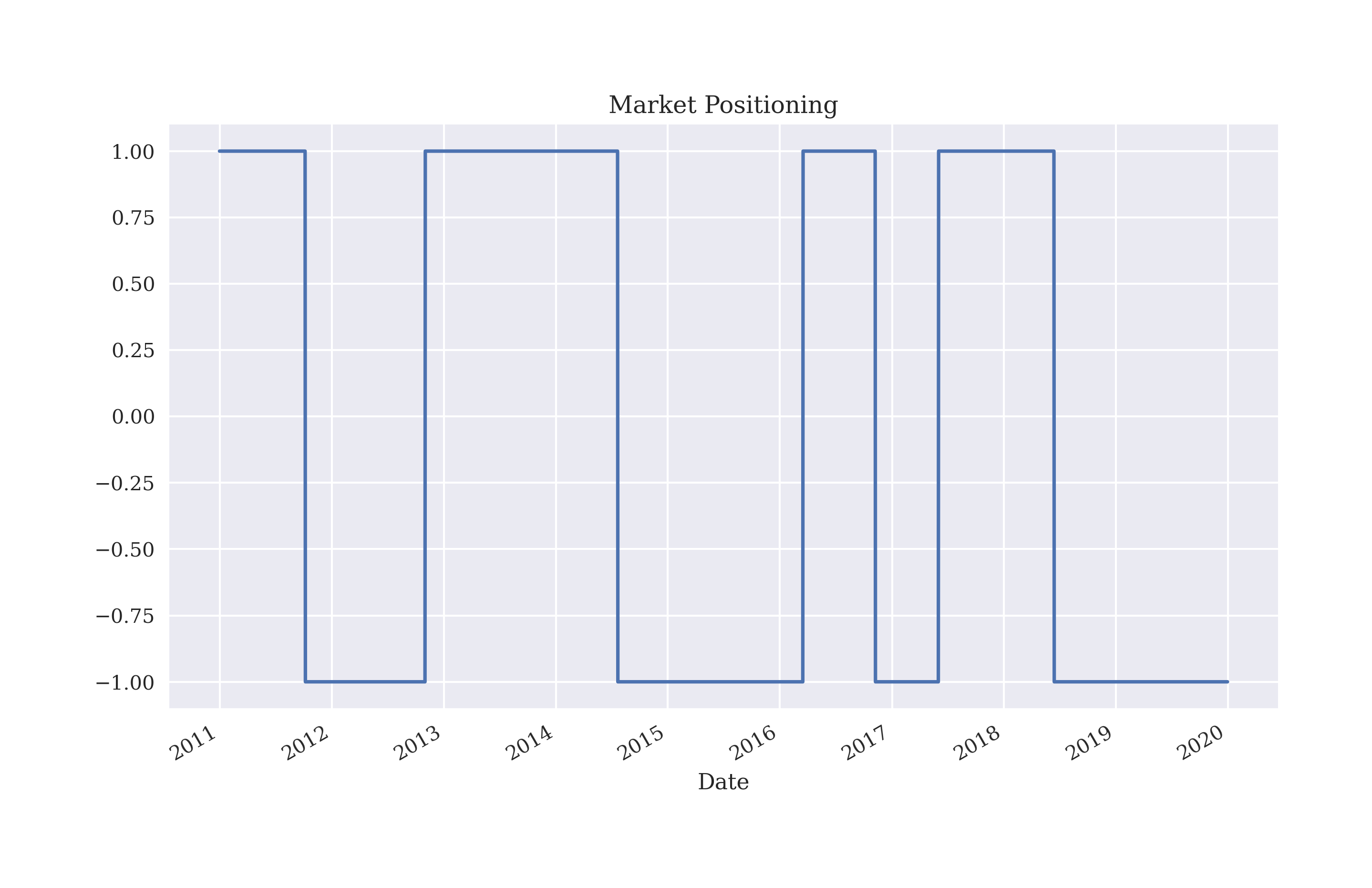
Figure 4-2. Market positioning based on the strategy with two SMAs

To calculate the performance of the strategy, calculate the log returns based on the original financial time series next. The code to do this is again rather concise due to vectorization. Figure 4-3 shows the histogram of the log returns.

In [50]: data['returns'] = np.log(data['price'] / data['price'].shift(1))  

In [51]: data['returns'].hist(bins=35, figsize=(10, 6));  

Calculates the log returns in vectorized fashion over the price column.

Plots the log returns as a histogram (frequency distribution).

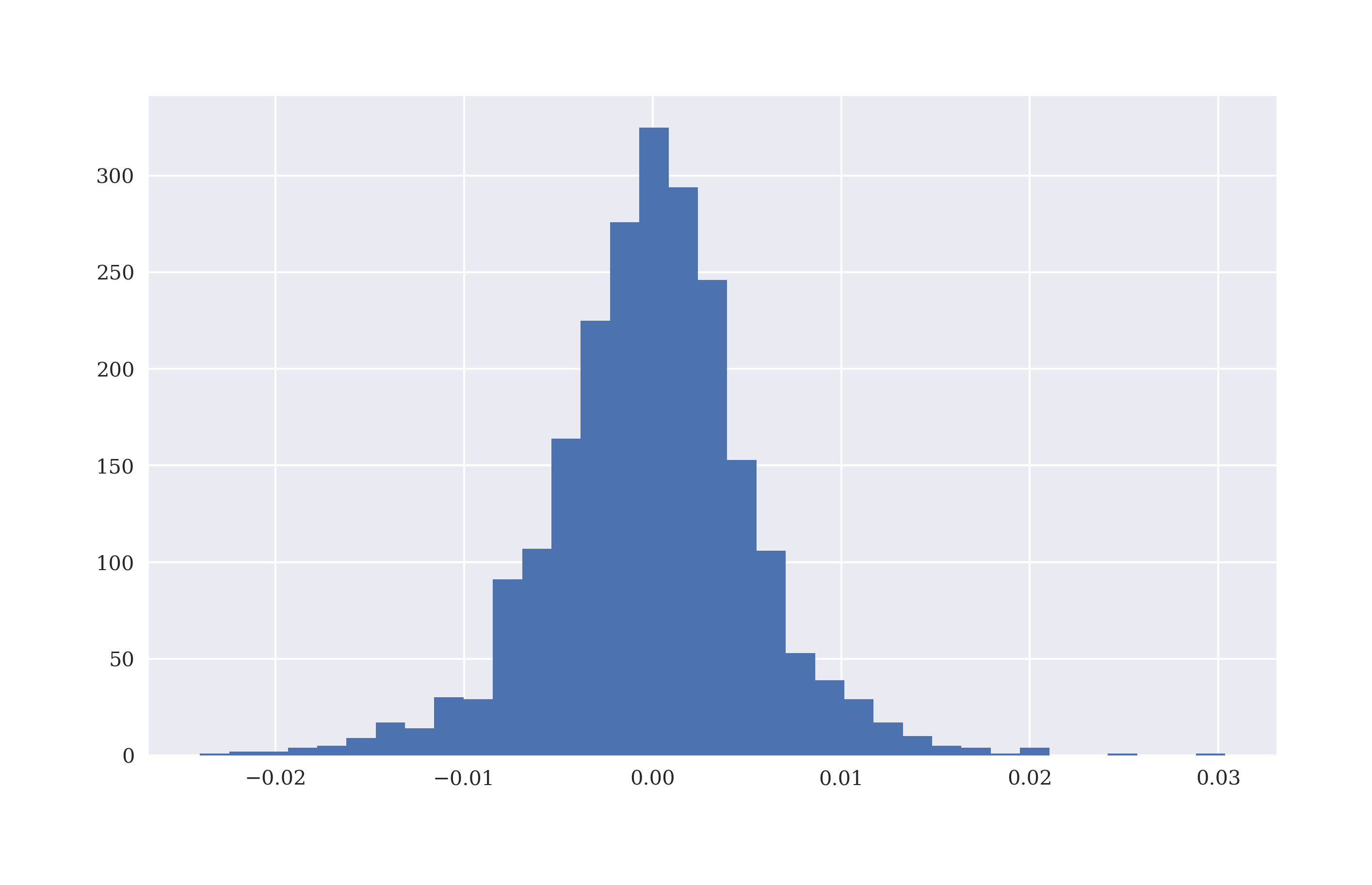
Figure 4-3. Frequency distribution of EUR/USD log returns

To derive the strategy returns, multiply the position column — shifted by one trading day — with the returns column. Since log returns are additive, calculating the sum over the columns returns and strategy provides a first comparison of the performance of the strategy relative to the base investment itself. Comparing the returns shows that the strategy books a win over the passive benchmark investment.

In [52]: data['strategy'] = data['position'].shift(1) * data['returns']  

In [53]: data[['returns', 'strategy']].sum()  
Out[53]: returns    -0.176731
         strategy    0.253121
         dtype: float64

In [54]: data[['returns', 'strategy']].sum().apply(np.exp)  
Out[54]: returns     0.838006
         strategy    1.288039
         dtype: float64

Derives the log returns of the strategy given the positionings and market returns.

Sums up the single log return values for both the stock and the strategy (for illustration only).

Applies the exponential function to the sum of the log returns to calculate the gross performance.

Calculating the cumulative sum over time with cumsum and based on this the cumulative returns by applying the exponential function np.exp() gives a more comprehensive picture of how the strategy compares to the performance of the base financial instrument over time. Figure 4-4 shows the data graphically and illustrates the outperformance in this particular case.

In [55]: data[['returns', 'strategy']].cumsum(
                     ).apply(np.exp).plot(figsize=(10, 6));

Figure 4-4. Gross performance of EUR/USD compared to the SMA-based strategy

Average, annualized risk-return statistics for both the stock and the strategy are easy to calculate.

In [56]: data[['returns', 'strategy']].mean() * 252  
Out[56]: returns    -0.019671
         strategy    0.028174
         dtype: float64

In [57]: np.exp(data[['returns', 'strategy']].mean() * 252) - 1  
Out[57]: returns    -0.019479
         strategy    0.028575
         dtype: float64

In [58]: data[['returns', 'strategy']].std() * 252 ** 0.5  
Out[58]: returns     0.085414
         strategy    0.085405
         dtype: float64

In [59]: (data[['returns', 'strategy']].apply(np.exp) - 1).std() * 252 ** 0.5  
Out[59]: returns     0.085405
         strategy    0.085373
         dtype: float64

Calculates the annualized mean return — in both log and regular space.

Calculates the annualized standard deviation — in both log and regular space.

Other risk statistics often of interest in the context of trading strategy performances are the maximum drawdown and the longest drawdown period. A helper statistic to use in this context is the cumulative maximum gross performance as calculated by the cummax() method applied to the gross performance of the strategy. Figure 4-5 shows the two time series for the SMA-based strategy.

In [60]: data['cumret'] = data['strategy'].cumsum().apply(np.exp)  

In [61]: data['cummax'] = data['cumret'].cummax()  

In [62]: data[['cumret', 'cummax']].dropna().plot(figsize=(10, 6));  

Defines a new column cumret with the gross performance over time.

Defines yet another column with the running maximum value of the gross performance.

This plots the two new columns of the DataFrame object.

Figure 4-5. Gross performance and cumulative maximum performance of the SMA-based strategy

The maximum drawdown is then simply calculated as the maximum of the difference between the two relevant columns. The maximum drawdown in the example is about 18 percentage points.

In [63]: drawdown = data['cummax'] - data['cumret']  

In [64]: drawdown.max()  
Out[64]: 0.17779367070195917

Calculates the element-wise difference between the two columns.

Picks out the maximum value from all differences.

The determination of the longest drawdown period is a bit more involved. It requires those dates at which the gross performance equals its cumulative maximum, that is where a new maximum is set. This information is stored in a temporary object. Then the differences in days between all such dates are calculated and the longest period is picked out. Such periods can be only one day long or more than 100 days. Here, the longest drawdown period lasts for 596 days — a pretty long period.²

In [65]: temp = drawdown[drawdown == 0]  

In [66]: periods = (temp.index[1:].to_pydatetime() -
                    temp.index[:-1].to_pydatetime())  

In [67]: periods[12:15]
Out[67]: array([datetime.timedelta(days=1), datetime.timedelta(days=1),
                datetime.timedelta(days=10)], dtype=object)

In [68]: periods.max()  
Out[68]: datetime.timedelta(days=596)

Where are the differences equal to zero?

Calculates the timedelta values between all index values.

Picks out the maximum timedelta value.

Vectorized backtesting with pandas is generally a rather efficient endeavor due to the capabilities of the package and the main DataFrame class. However, the interactive approach illustrated so far does not work well when one wishes to implement a larger backtesting program which, for example, optimizes the parameters of a SMA-based strategy. To this end, a more general approach is advisable.

Generalizing the Approach

“SMA Backtesting Class” presents a Python code that contains a class for the vectorized backtesting of SMA-based trading strategies. In a sense, it is a generalization of the approach introduced in the previous sub-section. It allows to define an instance of the SMAVectorBacktester class by providing the following parameters:

• symbol: RIC (instrument data) to be used

• SMA1: for the time window in days for the shorter SMA

• SMA2: for the time window in days for the longer SMA

• start: for the start date of the data selection

• end: for the end date of the data selection

The application itself is best illustrated by an interactive session that makes use of the class. The example first replicates the backtest implemented before based on EUR/USD exchange rate data. It then optimizes the SMA parameters for maximum gross performance. Based on the optimal parameters, it plots the resulting gross performance of the strategy compared to the base instrument over the relevant period of time.

In [69]: import SMAVectorBacktester as SMA  

In [70]: smabt = SMA.SMAVectorBacktester('EUR=', 42, 252,
                                         '2010-1-1', '2019-12-31')   

In [71]: smabt.run_strategy()  
Out[71]: (1.29, 0.45)

In [72]: %%time
         smabt.optimize_parameters((30, 50, 2),
                                   (200, 300, 2))  
         CPU times: user 3.76 s, sys: 15.8 ms, total: 3.78 s
         Wall time: 3.78 s

Out[72]: (array([ 48., 238.]), 1.5)

In [73]: smabt.plot_results()  

This imports the module as SMA.

An instance of the main class is instantiated.

Backtests the SMA-based strategy given the parameters during instantiation.

The optimize_parameters() method takes as input parameter ranges with step sizes and determines the optimal combination by a brute force approach.

The plot_results() method plots the strategy performance compared to the benchmark instrument given the currently stored parameter values (here from the optimization procedure).

The gross performance of the strategy with the original parametrization is 1.24 or 124%. The optimized strategy yields an absolute return of 1.44 or 144% for the parameter combination SMA1 = 48 and SMA2 = 238. Figure 4-6 shows the gross performance over time graphically, again compared to the performance of the base instrument which represents the benchmark.

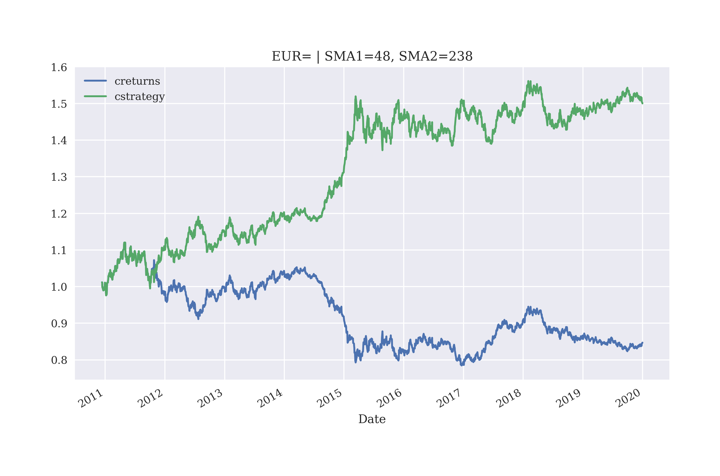
Figure 4-6. Gross returns of EUR/USD and the optimized SMA strategy

Getting into the Basics

Consider end-of-day closing prices for the for the gold price in USD (XAU=).

In [74]: data = pd.DataFrame(raw['XAU='])

In [75]: data.rename(columns={'XAU=': 'price'}, inplace=True)

In [76]: data['returns'] = np.log(data['price'] / data['price'].shift(1))

The most simple time series momentum strategy is to buy the stock if the last return was positive and to sell it if it was negative. With NumPy and pandas this is easy to formalize — just take the sign of the last available return as the market position. Figure 4-7 illustrates the performance of this strategy. The strategy does significantly underperform the base instrument.

In [77]: data['position'] = np.sign(data['returns'])  

In [78]: data['strategy'] = data['position'].shift(1) * data['returns']  

In [79]: data[['returns', 'strategy']].dropna().cumsum(
                     ).apply(np.exp).plot(figsize=(10, 6));  

Defines a new column with the sign, that is 1 or -1, of the relevant log return; the resulting values represent the market positionings (long or short).

Calculates the strategy log returns given the market positionings.

Plots and compares the strategy performance with the benchmark instrument.

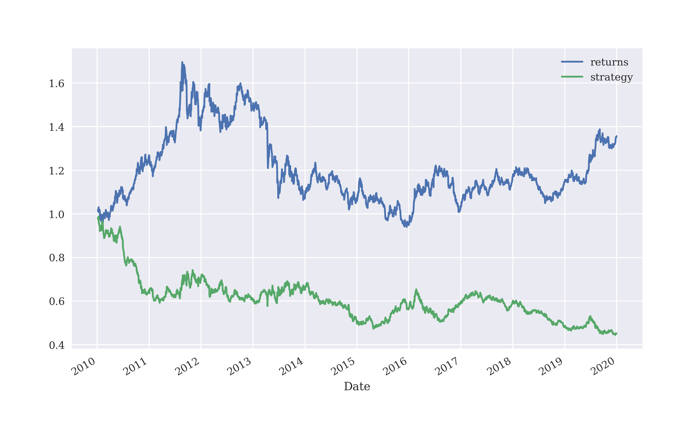
Figure 4-7. Gross performance of Gold price [USD] and momentum strategy (last return only)

Using a rolling time window, the time series momentum strategy can be generalized to more then just the last return. For example, the average of the last three returns can be used to generate the signal for the positioning. Figure 4-8 shows that the strategy in this case does much better — both in absolute terms and relative to the base instrument.

In [80]: data['position'] = np.sign(data['returns'].rolling(3).mean())  

In [81]: data['strategy'] = data['position'].shift(1) * data['returns']

In [82]: data[['returns', 'strategy']].dropna().cumsum(
                 ).apply(np.exp).plot(figsize=(10, 6));

This time, the mean return over a rolling window of three days is taken.

However, the performance is quite sensitive to the time window parameter. Choosing, for example, the last two returns instead of three leads to a much worse performance as shown in Figure 4-9

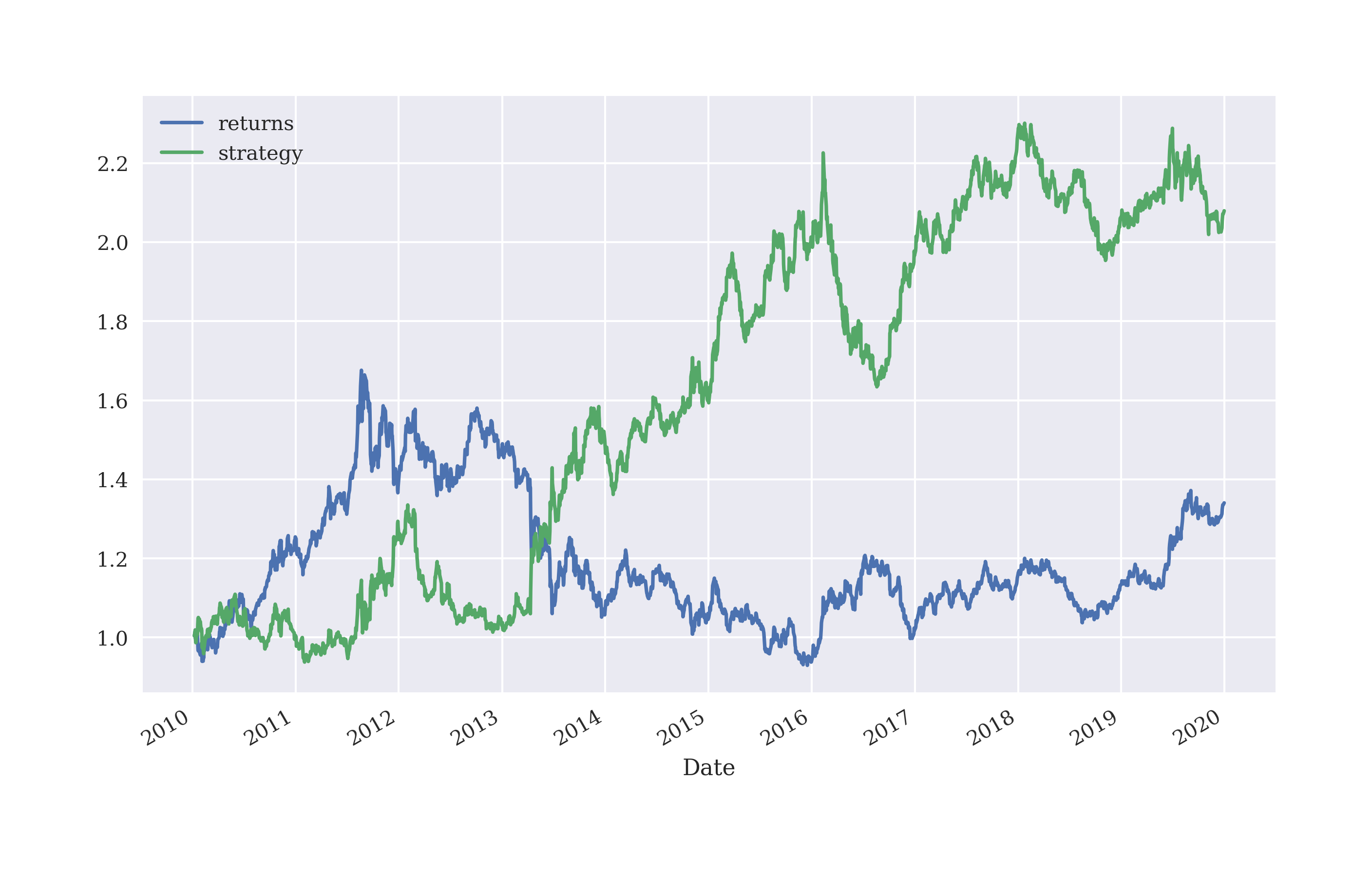
Figure 4-8. Gross performance of Gold price [USD] and momentum strategy (last three returns)

Figure 4-9. Gross performance of Gold price [USD] and momentum strategy (last two returns)

Time series momentum might be expected intraday as well. Actually, one would expect it to be more pronounced intraday the interday. Figure 4-10 shows the gross performance of five time series momentum strategies for one, three, five, seven, and nine return observations, respectively. The data used is intraday stock price data for Apple, Inc. as retrieved from the Eikon Data API. The figure is based on the code that follows. Basically all strategies outperform the stock over the course of this intraday time window, although some only slightly.

In [83]: fn = '../data/AAPL_1min_05052020.csv'  
         # fn = '../data/SPX_1min_05052020.csv'  # <1>#

In [84]: data = pd.read_csv(fn, index_col=0, parse_dates=True)  

In [85]: data.info()  
         <class 'pandas.core.frame.DataFrame'>
         DatetimeIndex: 241 entries, 2020-05-05 16:00:00 to 2020-05-05 20:00:00
         Data columns (total 6 columns):
          #   Column  Non-Null Count  Dtype
         ---  ------  --------------  -----
          0   HIGH    241 non-null    float64
          1   LOW     241 non-null    float64
          2   OPEN    241 non-null    float64
          3   CLOSE   241 non-null    float64
          4   COUNT   241 non-null    float64
          5   VOLUME  241 non-null    float64
         dtypes: float64(6)
         memory usage: 13.2 KB

In [86]: data['returns'] = np.log(data['CLOSE'] /
                                  data['CLOSE'].shift(1))  

In [87]: to_plot = ['returns']  

In [88]: for m in [1, 3, 5, 7, 9]:
             data['position_%d' % m] = np.sign(data['returns'].rolling(m).mean())  
             data['strategy_%d' % m] = (data['position_%d' % m].shift(1) *
                                        data['returns'])  
             to_plot.append('strategy_%d' % m)   

In [89]: data[to_plot].dropna().cumsum().apply(np.exp).plot(
             title='AAPL intraday 05. May 2020',
             figsize=(10, 6), style=['-', '--', '--', '--', '--', '--']);  

Reads the intraday data from a CSV file.

Calculates the intraday log returns.

Defines a list object to select the columns to be plotted later.

Derives positionings according to the momentum strategy parameter.

Calculates the resulting strategy log returns.

Appends the column name to the list object.

Plots all relevant columns to compare the strategies’ performances to the benchmark instrument’s performance.

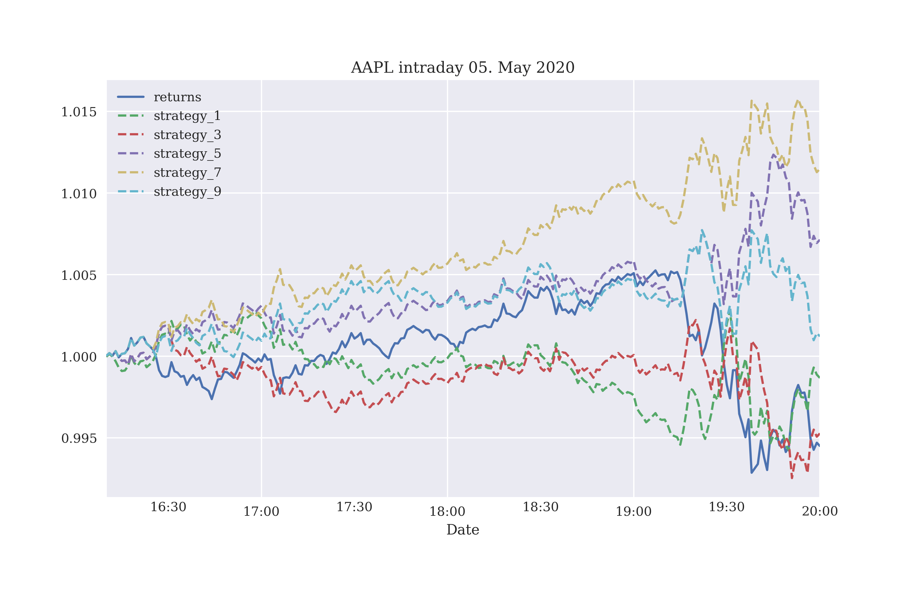
Figure 4-10. Gross intraday performance of the Apple stock and five momentum strategies (last one, three, five, seven, nine returns)

Figure 4-11 shows the performance of the same five strategies for the S&P 500 index. Again, all five strategy configurations outperform the index and all show a positive return (before transaction costs).

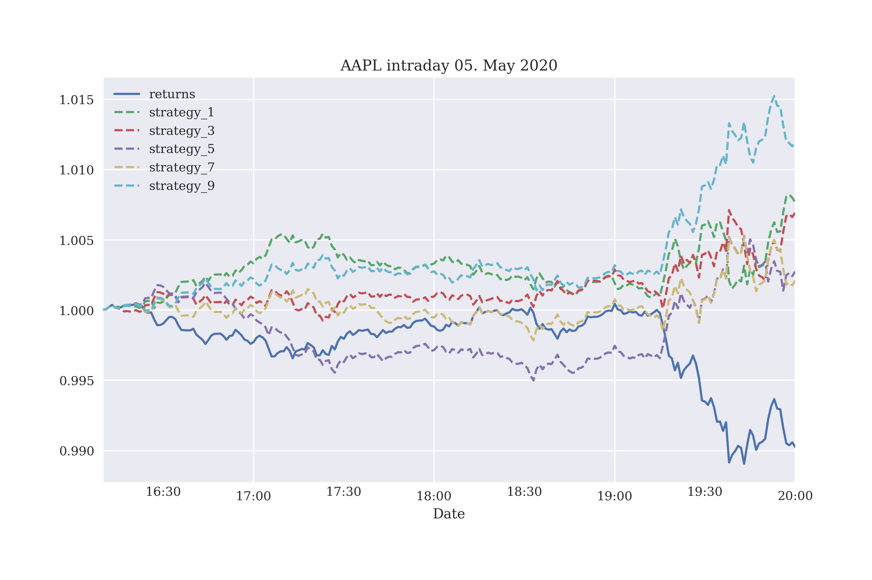
Figure 4-11. Gross intraday returns of the S&P 500 index and five momentum strategies (last one, three, five, seven, nine returns)

Generalizing the Approach

“Momentum Backtesting Class” presents a Python module containing the MomVectorBacktester class which allows for a bit more standardized backtesting of momentum-based strategies. The class has the following attributes:

• symbol: RIC (instrument data) to be used

• start: for the start date of the data selection

• end: for the end date of the data selection

• amount: for the initial amount to be invested

• tc: for the proportional transaction costs per trade

Compared to the SMAVectorBacktester class, this one introduces two important generalizations: the fixed amount to be invested at the beginning of the backtesting period and proportional transaction costs to get closer to market realities cost-wise. In particular the addition of transaction costs is important in the context of time series momentum strategies that lead often to a large number of transactions over time.

The application is as straightforward and convenient as before. The example first replicates the results from the interactive session before but this time with an initial investment of 10,000 USD. Figure 4-12 visualizes the performance of the strategy taking the mean of the last three returns to generate signals for the positioning. The second case covered is one with proportional transaction costs of 0.1% per trade. As Figure 4-13 illustrates, even small transaction costs deteriorate the performance significantly in this case. The driving factor in this regard is the relatively high frequency of trades that the strategy requires.

In [90]: import MomVectorBacktester as Mom  

In [91]: mombt = Mom.MomVectorBacktester('XAU=', '2010-1-1',
                                         '2019-12-31', 10000, 0.0)  

In [92]: mombt.run_strategy(momentum=3)  
Out[92]: (20797.87, 7395.53)

In [93]: mombt.plot_results()
In [94]: mombt = Mom.MomVectorBacktester('XAU=', '2010-1-1',
                                         '2019-12-31', 10000, 0.001)  

In [95]: mombt.run_strategy(momentum=3)  
Out[95]: (10749.4, -2652.93)

In [96]: mombt.plot_results()

Imports the module as Mom

Instantiates an object of the backtesting class defining the starting capital to be 10,000 USD and the proportional transaction costs to be zero.

Backtests the momentum strategy based on a time window of three days: the strategy outperforms the benchmark passive investment.

This time, proportional transaction costs of 0.1% are assumed per trade.

In that case, the strategy basically loses all the outperformance.

Figure 4-12. Gross performance of the Gold price [USD] and the momentum strategy (last three returns, no transaction costs)

Figure 4-13. Gross performance of the Gold price [USD] and the momentum strategy (last three returns, transaction costs of 0.1%)

Getting into the Basics

The examples to follow are for two different financial instruments for which one would expect significant mean reversion since they are both based on the gold price:

• GLD is the symbol for SPDR Gold Shares which is the largest physically backed exchange traded fund (ETF) for gold (cf. SPDR Gold Shares home page)

• GDX is the symbol for the VanEck Vectors Gold Miners ETF which invests in equity products to track the NYSE Arca Gold Miners Index (cf. VanEck Vectors Gold Miners overview page)

The example starts with GLD and implements a mean-reversion strategy on the basis of a SMA of 25 days and a threshold value of 3.5 for the absolute deviation of the current price to deviate from the SMA to signal a positioning. Figure 4-14 shows the differences between the current price as well as the positive and negative threshold value to generate sell and buy signals, respectively.

In [97]: data = pd.DataFrame(raw['GDX'])

In [98]: data.rename(columns={'GDX': 'price'}, inplace=True)

In [99]: data['returns'] = np.log(data['price'] /
                                  data['price'].shift(1))

In [100]: SMA = 25  

In [101]: data['SMA'] = data['price'].rolling(SMA).mean()  

In [102]: threshold = 3.5  

In [103]: data['distance'] = data['price'] - data['SMA']  

In [104]: data['distance'].dropna().plot(figsize=(10, 6), legend=True)  
          plt.axhline(threshold, color='r')
          plt.axhline(-threshold, color='r')
          plt.axhline(0, color='r');

The SMA parameter is defined …

… and SMA (“trend path”) is calculated.

The threshold for the signal generation is defined.

The distance is calculated for every point in time.

The distance values are plotted.

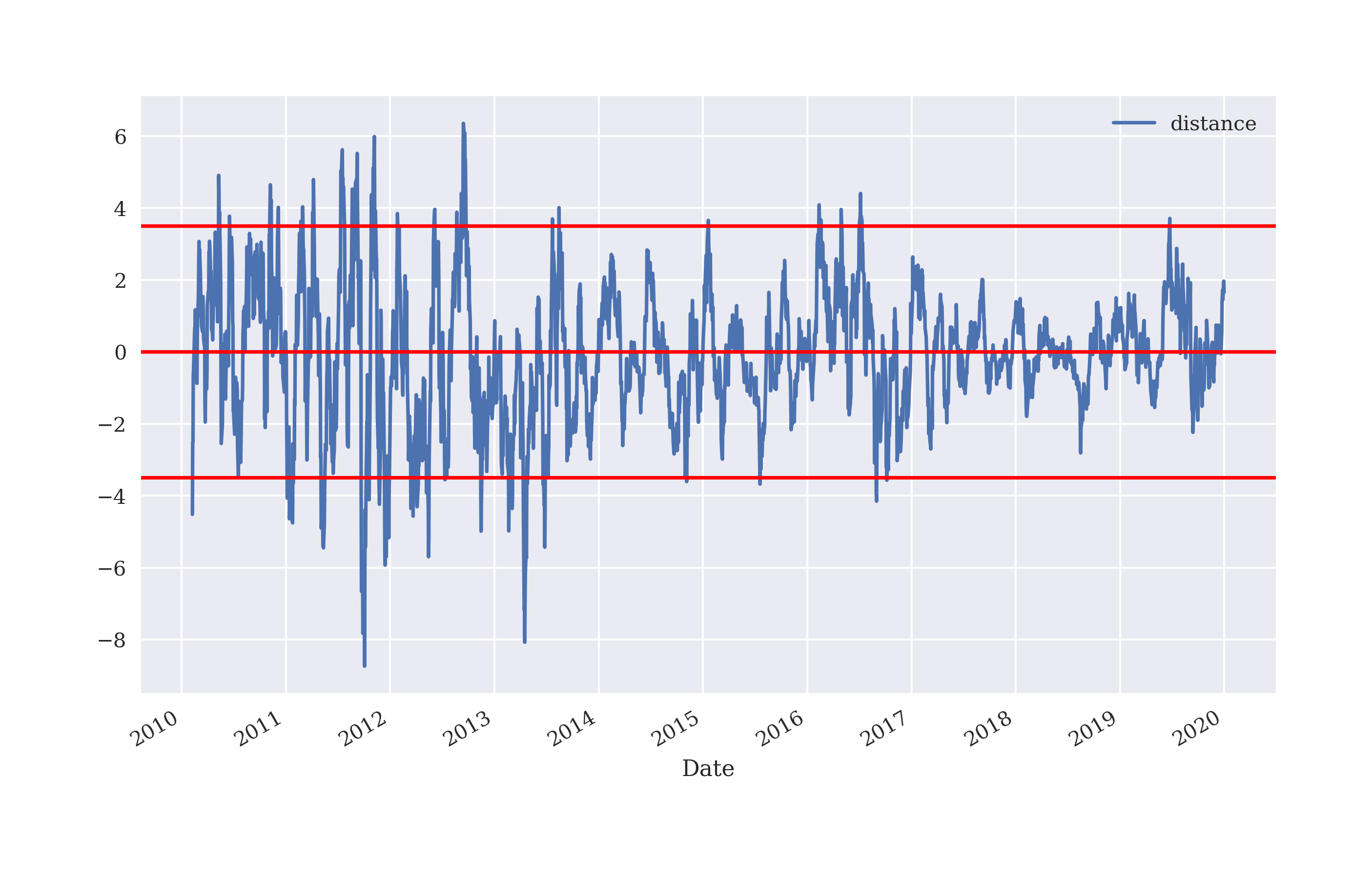
Figure 4-14. Difference between current price of GLD and SMA as well as threshold values for generating mean-reversion signals

Based on the differences and the fixed threshold values, positionings can again be derived in vectorized fashion. Figure 4-15 shows the resulting positionings.

In [105]: data['position'] = np.where(data['distance'] > threshold,
                                      -1, np.nan)  

In [106]: data['position'] = np.where(data['distance'] < -threshold,
                                      1, data['position'])  

In [107]: data['position'] = np.where(data['distance'] *
                      data['distance'].shift(1) < 0, 0, data['position'])  

In [108]: data['position'] = data['position'].ffill().fillna(0)  

In [109]: data['position'].iloc[SMA:].plot(ylim=[-1.1, 1.1],
                                         figsize=(10, 6));  

If the distance value is greater than the threshold value go short (set -1 in the new column position) otherwise set NaN.

If the distance value is lower than the negative threshold value go long (set 1), otherwise keep the column position unchanged.

If there is a change in the sign of the distance value go market neutral (set 0), otherwise keep the column position unchanged.

Forward fill all NaN position with the previous values; replace all remaining NaN values by 0.

Plot the resulting positionings from the index position SMA on.

Figure 4-15. Positionings generated for GLD based on the mean-reversion strategy

The final step is to derive the strategy returns that are shown in Figure 4-16. The strategy outperforms the GLD ETF by quite a margin although the particular parametrization leads to long periods with a neutral position (neither long or short). These neutral positions are reflected in the flat parts of the strategy curve in Figure 4-16.

In [110]: data['strategy'] = data['position'].shift(1) * data['returns']

In [111]: data[['returns', 'strategy']].dropna().cumsum(
                  ).apply(np.exp).plot(figsize=(10, 6));

Figure 4-16. Gross performance of the GLD ETF and the mean-reversion strategy (SMA = 25, threshold = 3.5)

Generalizing the Approach

As before, the vectorized backtesting is more efficient to implement based on a respective Python class. The class MRVectorBacktester presented in “Mean Reversion Backtesting Class” inherits from the MomVectorBacktester class and just replaces the run_strategy() method to accommodate for the specifics of the mean-reversion strategy.

The example now uses GDX and sets the proportional transaction costs to 0.1%. The initial amount to invest is again set to 10,000 USD. The SMA is 43 this time and the threshold value is set to 7.5. Figure 4-17 shows the performance of the mean-reversion strategy compared to the GDX ETF.

In [112]: import MRVectorBacktester as MR  

In [113]: mrbt = MR.MRVectorBacktester('GLD', '2010-1-1', '2019-12-31',
                                       10000, 0.001)  

In [114]: mrbt.run_strategy(SMA=43, threshold=7.5)  
Out[114]: (13542.15, 646.21)

In [115]: mrbt.plot_results()  

Imports the module as MR.

Instantiates an object of the MRVectorBacktester class with 10,000 USD initial capital and 0.1% proportional transaction costs per trade; the strategy significantly outperforms the benchmark instrument in this case.

Backtests the mean-reversion strategy with an SMA value of 43 and a threshold value of 7.5.

Plots the cumulative performance of the strategy against the base instrument.

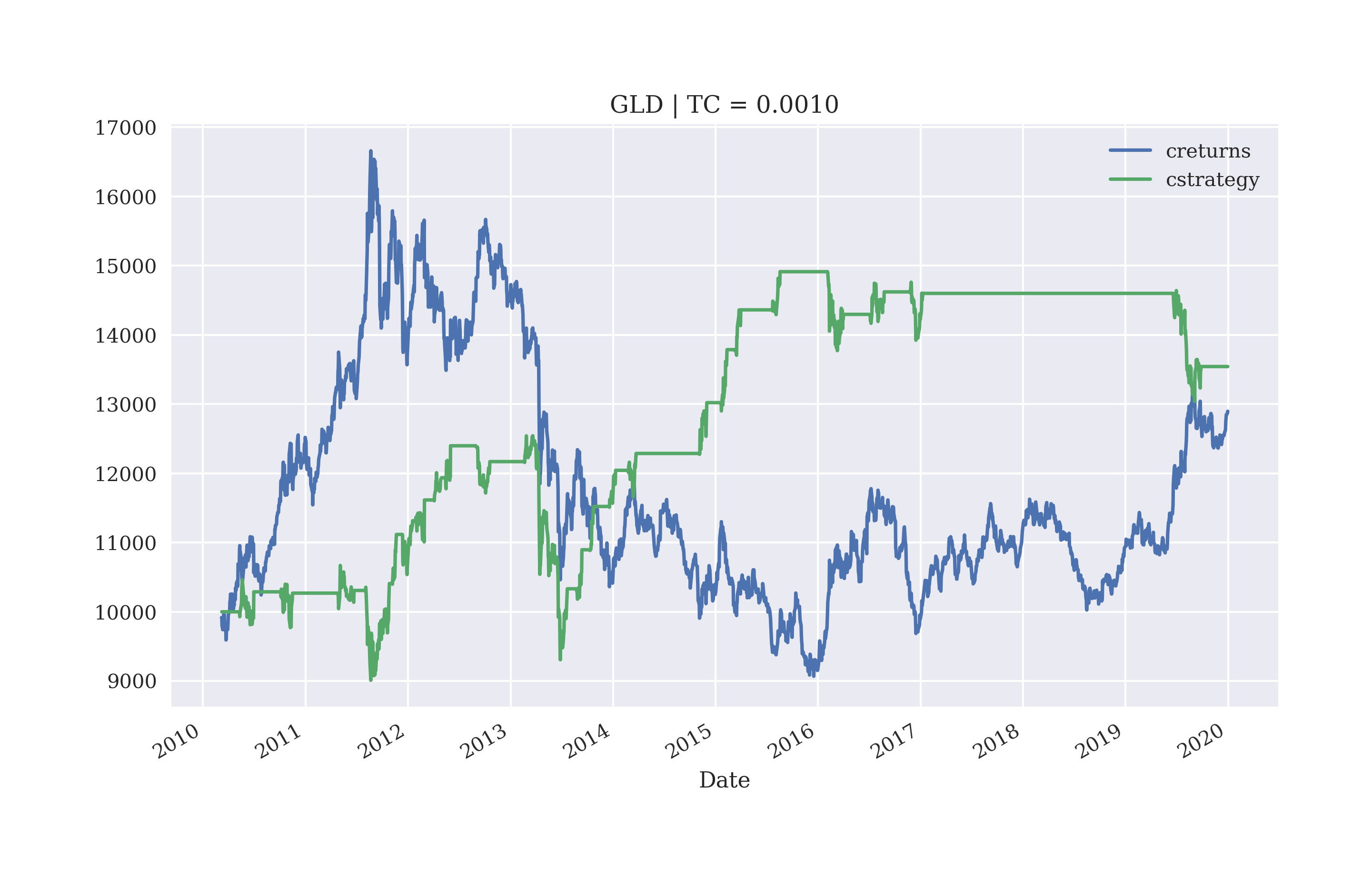
Figure 4-17. Gross performance of the GLD ETF and the mean-reversion strategy (SMA = 43, threshold = 7.5, transaction costs of 0.1%)

SMA Backtesting Class

The following presents Python code with a class for the vectorized backtesting of strategies based on simple moving averages.

#
# Python Module with Class
# for Vectorized Backtesting
# of SMA-based Strategies
#
# Python for Algorithmic Trading
# (c) Dr. Yves J. Hilpisch
# The Python Quants GmbH
#
import numpy as np
import pandas as pd
from scipy.optimize import brute


class SMAVectorBacktester(object):
    ''' Class for the vectorized backtesting of SMA-based trading strategies.

    Attributes
    ==========
    symbol: str
        RIC symbol with which to work with
    SMA1: int
        time window in days for shorter SMA
    SMA2: int
        time window in days for longer SMA
    start: str
        start date for data retrieval
    end: str
        end date for data retrieval

    Methods
    =======
    get_data:
        retrieves and prepares the base data set
    set_parameters:
        sets one or two new SMA parameters
    run_strategy:
        runs the backtest for the SMA-based strategy
    plot_results:
        plots the performance of the strategy compared to the symbol
    update_and_run:
        updates SMA parameters and returns the (negative) absolute performance
    optimize_parameters:
        implements a brute force optimizeation for the two SMA parameters
    '''

    def __init__(self, symbol, SMA1, SMA2, start, end):
        self.symbol = symbol
        self.SMA1 = SMA1
        self.SMA2 = SMA2
        self.start = start
        self.end = end
        self.results = None
        self.get_data()

    def get_data(self):
        ''' Retrieves and prepares the data.
        '''
        raw = pd.read_csv('http://hilpisch.com/pyalgo_eikon_eod_data.csv',
                          index_col=0, parse_dates=True).dropna()
        raw = pd.DataFrame(raw[self.symbol])
        raw = raw.loc[self.start:self.end]
        raw.rename(columns={self.symbol: 'price'}, inplace=True)
        raw['return'] = np.log(raw / raw.shift(1))
        raw['SMA1'] = raw['price'].rolling(self.SMA1).mean()
        raw['SMA2'] = raw['price'].rolling(self.SMA2).mean()
        self.data = raw

    def set_parameters(self, SMA1=None, SMA2=None):
        ''' Updates SMA parameters and resp. time series.
        '''
        if SMA1 is not None:
            self.SMA1 = SMA1
            self.data['SMA1'] = self.data['price'].rolling(
                self.SMA1).mean()
        if SMA2 is not None:
            self.SMA2 = SMA2
            self.data['SMA2'] = self.data['price'].rolling(self.SMA2).mean()

    def run_strategy(self):
        ''' Backtests the trading strategy.
        '''
        data = self.data.copy().dropna()
        data['position'] = np.where(data['SMA1'] > data['SMA2'], 1, -1)
        data['strategy'] = data['position'].shift(1) * data['return']
        data.dropna(inplace=True)
        data['creturns'] = data['return'].cumsum().apply(np.exp)
        data['cstrategy'] = data['strategy'].cumsum().apply(np.exp)
        self.results = data
        # gross performance of the strategy
        aperf = data['cstrategy'].iloc[-1]
        # out-/underperformance of strategy
        operf = aperf - data['creturns'].iloc[-1]
        return round(aperf, 2), round(operf, 2)

    def plot_results(self):
        ''' Plots the cumulative performance of the trading strategy
        compared to the symbol.
        '''
        if self.results is None:
            print('No results to plot yet. Run a strategy.')
        title = '%s | SMA1=%d, SMA2=%d' % (self.symbol,
                                               self.SMA1, self.SMA2)
        self.results[['creturns', 'cstrategy']].plot(title=title,
                                                     figsize=(10, 6))

    def update_and_run(self, SMA):
        ''' Updates SMA parameters and returns negative absolute performance
        (for minimazation algorithm).

        Parameters
        ==========
        SMA: tuple
            SMA parameter tuple
        '''
        self.set_parameters(int(SMA[0]), int(SMA[1]))
        return -self.run_strategy()[0]

    def optimize_parameters(self, SMA1_range, SMA2_range):
        ''' Finds global maximum given the SMA parameter ranges.

        Parameters
        ==========
        SMA1_range, SMA2_range: tuple
            tuples of the form (start, end, step size)
        '''
        opt = brute(self.update_and_run, (SMA1_range, SMA2_range), finish=None)
        return opt, -self.update_and_run(opt)


if __name__ == '__main__':
    smabt = SMAVectorBacktester('EUR=', 42, 252,
                                '2010-1-1', '2020-12-31')
    print(smabt.run_strategy())
    smabt.set_parameters(SMA1=20, SMA2=100)
    print(smabt.run_strategy())
    print(smabt.optimize_parameters((30, 56, 4), (200, 300, 4)))

Momentum Backtesting Class

The following presents Python code with a class for the vectorized backtesting of strategies based on time series momentum.

#
# Python Module with Class
# for Vectorized Backtesting
# of Momentum-based Strategies
#
# Python for Algorithmic Trading
# (c) Dr. Yves J. Hilpisch
# The Python Quants GmbH
#
import numpy as np
import pandas as pd


class MomVectorBacktester(object):
    ''' Class for the vectorized backtesting of
    Momentum-based trading strategies.

    Attributes
    ==========
    symbol: str
       RIC (financial instrument) to work with
    start: str
        start date for data selection
    end: str
        end date for data selection
    amount: int, float
        amount to be invested at the beginning
    tc: float
        proportional transaction costs (e.g. 0.5% = 0.005) per trade

    Methods
    =======
    get_data:
        retrieves and prepares the base data set
    run_strategy:
        runs the backtest for the momentum-based strategy
    plot_results:
        plots the performance of the strategy compared to the symbol
    '''

    def __init__(self, symbol, start, end, amount, tc):
        self.symbol = symbol
        self.start = start
        self.end = end
        self.amount = amount
        self.tc = tc
        self.results = None
        self.get_data()

    def get_data(self):
        ''' Retrieves and prepares the data.
        '''
        raw = pd.read_csv('http://hilpisch.com/pyalgo_eikon_eod_data.csv',
                          index_col=0, parse_dates=True).dropna()
        raw = pd.DataFrame(raw[self.symbol])
        raw = raw.loc[self.start:self.end]
        raw.rename(columns={self.symbol: 'price'}, inplace=True)
        raw['return'] = np.log(raw / raw.shift(1))
        self.data = raw

    def run_strategy(self, momentum=1):
        ''' Backtests the trading strategy.
        '''
        self.momentum = momentum
        data = self.data.copy().dropna()
        data['position'] = np.sign(data['return'].rolling(momentum).mean())
        data['strategy'] = data['position'].shift(1) * data['return']
        # determine when a trade takes place
        data.dropna(inplace=True)
        trades = data['position'].diff().fillna(0) != 0
        # subtract transaction costs from return when trade takes place
        data['strategy'][trades] -= self.tc
        data['creturns'] = self.amount * data['return'].cumsum().apply(np.exp)
        data['cstrategy'] = self.amount * 
            data['strategy'].cumsum().apply(np.exp)
        self.results = data
        # absolute performance of the strategy
        aperf = self.results['cstrategy'].iloc[-1]
        # out-/underperformance of strategy
        operf = aperf - self.results['creturns'].iloc[-1]
        return round(aperf, 2), round(operf, 2)

    def plot_results(self):
        ''' Plots the cumulative performance of the trading strategy
        compared to the symbol.
        '''
        if self.results is None:
            print('No results to plot yet. Run a strategy.')
        title = '%s | TC = %.4f' % (self.symbol, self.tc)
        self.results[['creturns', 'cstrategy']].plot(title=title,
                                                     figsize=(10, 6))


if __name__ == '__main__':
    mombt = MomVectorBacktester('XAU=', '2010-1-1', '2020-12-31',
                                10000, 0.0)
    print(mombt.run_strategy())
    print(mombt.run_strategy(momentum=2))
    mombt = MomVectorBacktester('XAU=', '2010-1-1', '2020-12-31',
                                10000, 0.001)
    print(mombt.run_strategy(momentum=2))