Chapter 5. Predicting Market Movements with Machine Learning
Skynet begins to learn at a geometric rate. It becomes self-aware at 2:14 a.m. Eastern time, August 29th.
The Terminator (Terminator 2)
Recent years have seen tremendous progress in the areas of machine learning, deep learning and artificial intelligence. The financial industry in general and algorithmic traders around the globe in particular also try to benefit from these technological advances. This chapter introduces techniques from statistics, like linear regression, and machine learning, like logistic regression, to predict future price movements based on past returns. It also illustrates the use of neural networks to predict stock market movements. This chapter can of course not replace a thorough introduction to machine learning but it can show, from a practitioner’s point of view, how to concretely apply certain techniques to the price prediction problem. For more details, refer to Hilpisch (2020).1
The chapter covers the following types of trading strategies:
-
Linear regression-based strategies: Such strategies use linear regression to extrapolate a trend or to derive a financial instrument’s direction of future price movement.
-
Machine learning-based strategies: In algorithmic trading it is generally enough to predict the direction of movement for a financial instrument as opposed to the absolute magnitude of that movement. With this reasoning, the prediction problem boils basically down to a classification problem of deciding whether there will be an upwards or downwards movement. Different machine learning algorithms have been developed to attack such classification problems. This chapter introduces logistic regression, as a typical baseline algorithm, for classification.
-
Deep learning-based strategies: Deep learning has been popularized by such technological giants as or Facebook. Similar to machine learning algorithms, deep learning algorithms based on neural networks allow to attack classification problems faced in financial market prediction.
The chapter is organized as follow. “Using Linear Regression for Market Movement Prediction” introduces linear regression as a technique to predict index levels and the direction of price movements. “Using Machine Learning for Market Movement Prediction” focuses on machine learning and introduces scikit-learn on the basis of linear regression. It mainly covers logistic regression as an alternative linear model explicitly applicable to classification problems. “Using Deep Learning for Market Movement Prediction” introduces Keras to predict the direction of stock market movements based on neural network algorithms.
The major goal of this chapter is to provide practical approaches to predict future price movements in financial markets based on past returns. The basic assumption is that the efficient market hypothesis does not hold universally and that — similar to the reasoning behind the technical analysis of stock price charts — the history might provide some insights about the future that can be mined with statistical techniques. In other words, it is assumed that certain patterns in financial markets repeat themselves such that past observations can be leveraged to predict future price movements. More details are covered in Hilpisch (2020).
Using Linear Regression for Market Movement Prediction
Ordinary least squares (OLS) and linear regression are decades-old statistical techniques that have proven useful in many different application areas. This section uses linear regression for price prediction purposes. However, it starts with a quick review of the basics and an introduction to the basic approach.
A Quick Review of Linear Regression
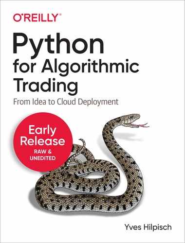
Before applying linear regression, a quick review of the approach based on some randomized data might be helpful. The example code uses NumPy to first generate a ndarray object with data for the independent variable x. Based on this data, randomized data (“noisy data”) for the dependent variable y is generated. NumPy provides two functions, polyfit and polyval, for a convenient implementation of OLS regression based on simple monomials. For a linear regression the highest degree for the monomials to be used is set to 1. Figure 5-1 shows the data and the regression line.
In[1]:importosimportrandomimportnumpyasnpfrompylabimportmpl,pltplt.style.use('seaborn')mpl.rcParams['savefig.dpi']=300mpl.rcParams['font.family']='serif'os.environ['PYTHONHASHSEED']='0'In[2]:x=np.linspace(0,10)In[3]:defset_seeds(seed=100):random.seed(seed)np.random.seed(seed)set_seeds()In[4]:y=x+np.random.standard_normal(len(x))In[5]:reg=np.polyfit(x,y,deg=1)In[6]:regOut[6]:array([0.94612934,0.22855261])In[7]:plt.figure(figsize=(10,6))plt.plot(x,y,'bo',label='data')plt.plot(x,np.polyval(reg,x),'r',lw=2.5,label='linear regression')plt.legend(loc=0);

Import
NumPy…
… and
matplotlib.
Generates an evenly spaced grid of floats for the
xvalues between 0 and 10.
Fixes the seed values for the all relevant random number generators.

Generates the randomized data for the
yvalues.
OLS regression of degree 1, i.e. linear regression, is conducted.

Shows the optimal parameter values.

Creates a new figure object.

Plots the original data set as dots.

Plots the regression line.

Creates the legend.

Figure 5-1. Linear regression illustrated based on randomized data
The interval for the dependent variable x is . Enlarging the interval to, say, allows to “predict” values for the dependent variable y beyond the domain of the original data set by an extrapolation given the optimal regression parameters. Figure 5-2 visualizes the extrapolation.
In[8]:plt.figure(figsize=(10,6))plt.plot(x,y,'bo',label='data')xn=np.linspace(0,20)plt.plot(xn,np.polyval(reg,xn),'r',lw=2.5,label='linear regression')plt.legend(loc=0);
Generates an enlarged domain for the
xvalues.
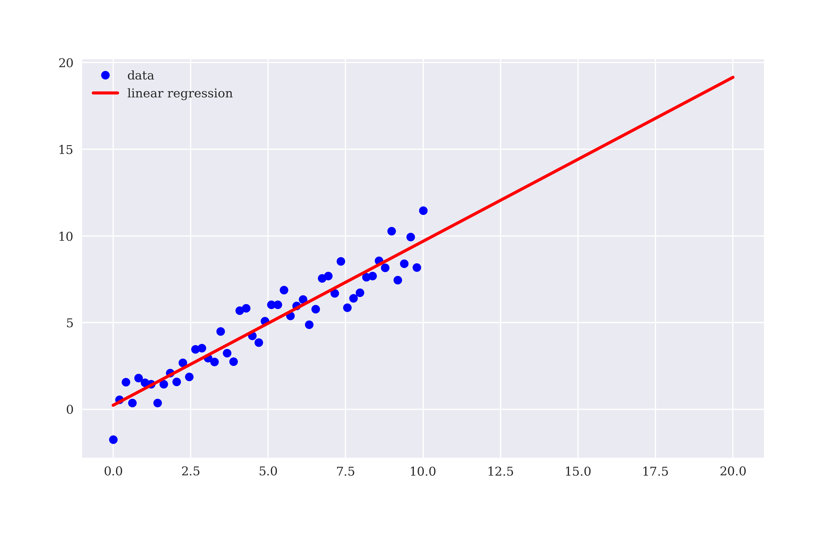
Figure 5-2. Prediction (extrapolation) based on linear regression
The Basic Idea for Price Prediction
Price prediction based on time series data has to deal with one special feature: the time-based ordering of the data. Generally, the ordering of the data is not important for the application of linear regression. In the first example above, the data on which the linear regression is implemented could have been compiled in completely different orderings — while keeping the x and y pairs constant. Independent of the ordering, the optimal regression parameters would have been the same.
In the context of predicting tomorrow’s index level, for example, it seems to be, however, of paramount importance to have the historic index levels in the correct order. If this is the case, one would then try to predict tomorrow’s index level given the index level of today, yesterday, the day before, etc. The number of days used as input is generally called lags. Using today’s index level and the two more from before therefore translates into three lags.
The next example casts this idea again into a rather simple context. The data the example uses are the numbers from 0 to 11.
In[9]:x=np.arange(12)In[10]:xOut[10]:array([0,1,2,3,4,5,6,7,8,9,10,11])
Assume three lags for the regression. This implies three independent variables for the regression and one dependent one. More concretely, 0, 1 and 2 are values of the independent variables while 3 would be the corresponding value for the dependent variable. Moving forward on step (“in time”), the values are 1, 2, and 3 as well as 4. The final combination of values is 8, 9 and 10 with 11. The problem therefore is to cast this idea formally into a linear equation of the form where is a matrix and and are vectors.
In[11]:lags=3In[12]:m=np.zeros((lags+1,len(x)-lags))In[13]:m[lags]=x[lags:]foriinrange(lags):m[i]=x[i:i-lags]In[14]:m.TOut[14]:array([[0.,1.,2.,3.],[1.,2.,3.,4.],[2.,3.,4.,5.],[3.,4.,5.,6.],[4.,5.,6.,7.],[5.,6.,7.,8.],[6.,7.,8.,9.],[7.,8.,9.,10.],[8.,9.,10.,11.]])
Defines the number of lags.
Instantiates an
ndarrayobject with the appropriate dimensions.Defines the target values (dependent variable).
Iterates over the numbers from
0tolags - 1.Defines the basis vectors (independent variables)
Shows the transpose of the
ndarrayobjectm.
In the transposed ndarray object m, the first three columns contain the values for the three independent variables. They together form the matrix . The fourth and final column represents the vector . Linear regression then yields as a result the missing vector . Since there are now more independent variables, polyfit and polyval do not work anymore. However, there is a function in the NumPy sub-package for linear algebra (linalg) that allows to solve general least-squares problems: lstsq. Only the first element of the results array is needed since it contains the optimal regression parameters.
In[15]:reg=np.linalg.lstsq(m[:lags].T,m[lags],rcond=None)[0]In[16]:regOut[16]:array([-0.66666667,0.33333333,1.33333333])In[17]:np.dot(m[:lags].T,reg)Out[17]:array([3.,4.,5.,6.,7.,8.,9.,10.,11.])
Implements the linear OLS regression.
Prints out the optimal parameters.
The
dotproduct yields the prediction results.
This basic idea easily carries over to real world financial time series data.
Predicting Index Levels
The next step is to translate the basic approach to time series data for a real financial instrument, like the EUR/USD exchange rate.
In[18]:importpandasaspdIn[19]:raw=pd.read_csv('http://hilpisch.com/pyalgo_eikon_eod_data.csv',index_col=0,parse_dates=True).dropna()In[20]:raw.info()<class'pandas.core.frame.DataFrame'>DatetimeIndex:2516entries,2010-01-04to2019-12-31Datacolumns(total12columns):# Column Non-Null Count Dtype----------------------------0AAPL.O2516non-nullfloat641MSFT.O2516non-nullfloat642INTC.O2516non-nullfloat643AMZN.O2516non-nullfloat644GS.N2516non-nullfloat645SPY2516non-nullfloat646.SPX2516non-nullfloat647.VIX2516non-nullfloat648EUR=2516non-nullfloat649XAU=2516non-nullfloat6410GDX2516non-nullfloat6411GLD2516non-nullfloat64dtypes:float64(12)memoryusage:255.5KBIn[21]:symbol='EUR='In[22]:data=pd.DataFrame(raw[symbol])In[23]:data.rename(columns={symbol:'price'},inplace=True)
Imports the
pandaspackage.Retrieves end-of-day (EOD) data and stores it in a
DataFrameobject.The time series data for the specified symbol is selected from the original
DataFrame.Renames the single column to
price.
Formally, the Python code from the simple example before hardly needs to be changed to implement the regression-based prediction approach. Just the data object needs to be replaced.
In[24]:lags=5In[25]:cols=[]forlaginrange(1,lags+1):col=f'lag_{lag}'data[col]=data['price'].shift(lag)cols.append(col)data.dropna(inplace=True)In[26]:reg=np.linalg.lstsq(data[cols],data['price'],rcond=None)[0]In[27]:regOut[27]:array([0.98635864,0.02292172,-0.04769849,0.05037365,-0.01208135])
Takes now the
pricecolumn and shifts it bylag.
The optimal regression parameters illustrate what is typically called the random walk hypothesis. This hypothesis states that stock prices or exchange rates, for example, follow a random walk with the consequence that the best predictor for tomorrow’s price is today’s price. The optimal parameters seem to support such a hypothesis since today’s price almost completely explains the predicted price level for tomorrow. The four other values hardly have any weight assigned.
Figure 5-3 shows the EUR/USD exchange rate and the predicted values. Due to the sheer amount of data for the multi-year time window the two time series are indistinguishable in the plot.
In[28]:data['prediction']=np.dot(data[cols],reg)In[29]:data[['price','prediction']].plot(figsize=(10,6));
Calculates the prediction values as the
dotproduct.Plots the
priceandpredictioncolumns.
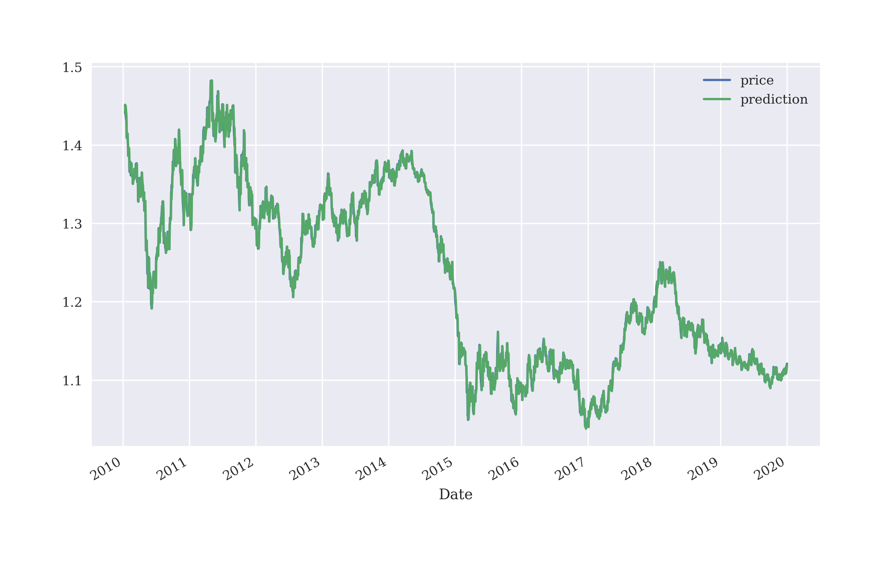
Figure 5-3. EUR/USD exchange rate and predicted values based on linear regression (5 lags)
Zooming in by plotting the results for a much shorter time window, allows to better distinguish the two time series. Figure 5-4 shows the results for a three months time window. This plot illustrates that the prediction for tomorrow’s rate is roughly today’s rate. The prediction is more or less a shift of the original rate to the right by one trading day.
In[30]:data[['price','prediction']].loc['2019-10-1':].plot(figsize=(10,6));
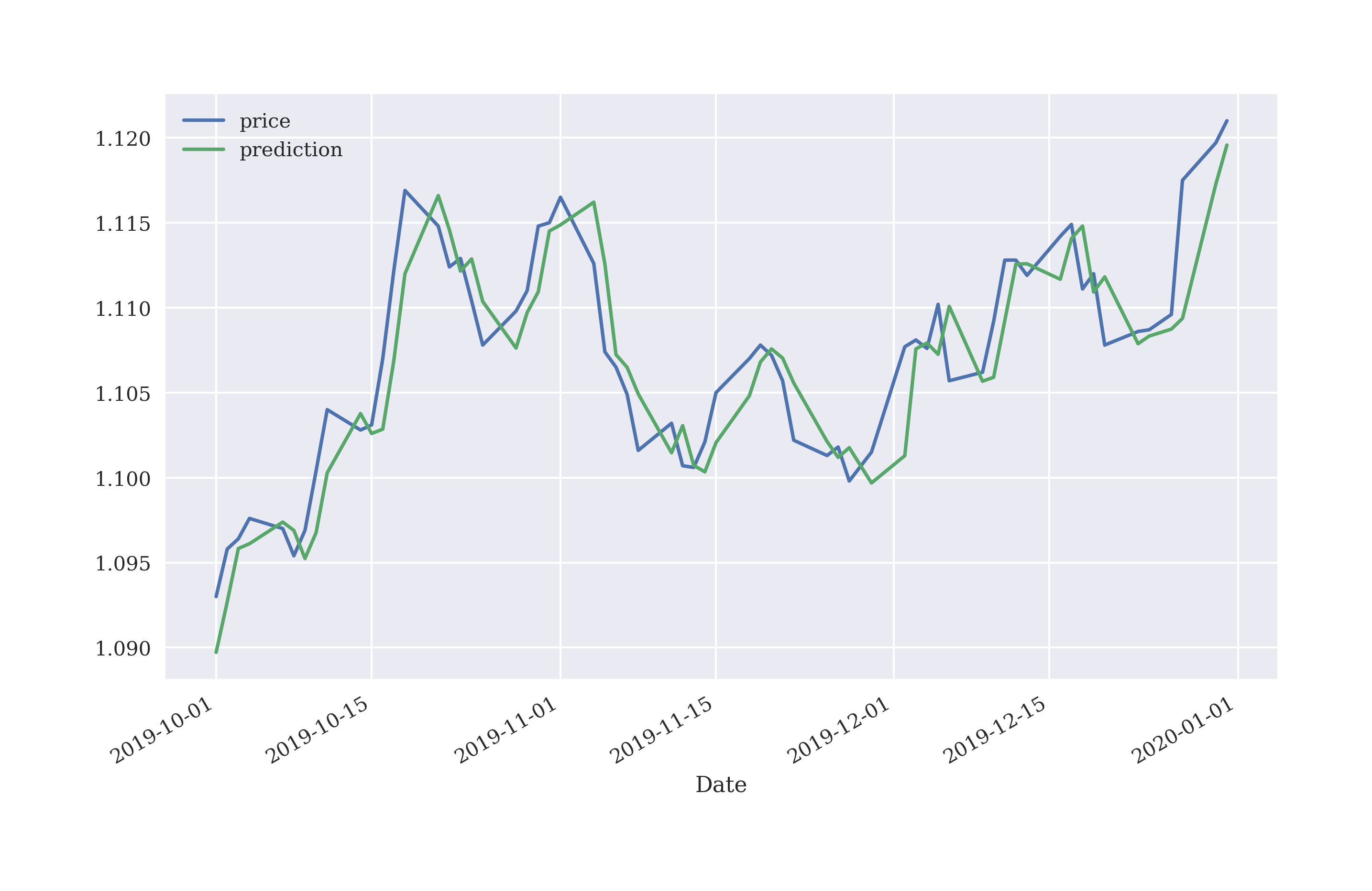
Figure 5-4. EUR/USD exchange rate and predicted values based on linear regression (5 lags, 3 months only)
Note
Applying linear OLS regression to predict rates for EUR/USD based on historical rates provides support for the random walk hypothesis. The results of the numerical example show that today’s rate is the best predictor for tomorrow’s rate in a least-squares sense.
Predicting Future Returns
So far, the analysis is based on absolute rate levels. However, (log) returns might be a better choice for such statistical applications due, for example, to their characteristic of making the time series data stationary. The code to apply linear regression to the returns data is almost the same as before. This time it is not only today’s return that is relevant to predict tomorrow’s return, the regression results are completely different in nature.
In[31]:data['return']=np.log(data['price']/data['price'].shift(1))In[32]:data.dropna(inplace=True)In[33]:cols=[]forlaginrange(1,lags+1):col=f'lag_{lag}'data[col]=data['return'].shift(lag)cols.append(col)data.dropna(inplace=True)In[34]:reg=np.linalg.lstsq(data[cols],data['return'],rcond=None)[0]In[35]:regOut[35]:array([-0.015689,0.00890227,-0.03634858,0.01290924,-0.00636023])
Calculates the log returns.
Deletes all lines with
NaNvalues.Takes now the
returnscolumn for the lagged data.
Figure 5-5 shows the returns data and the prediction values. As the figure impressively illustrates, linear regression can obviously not predict the magnitude of future returns to some significant extent.
In[36]:data['prediction']=np.dot(data[cols],reg)In[37]:data[['return','prediction']].iloc[lags:].plot(figsize=(10,6));
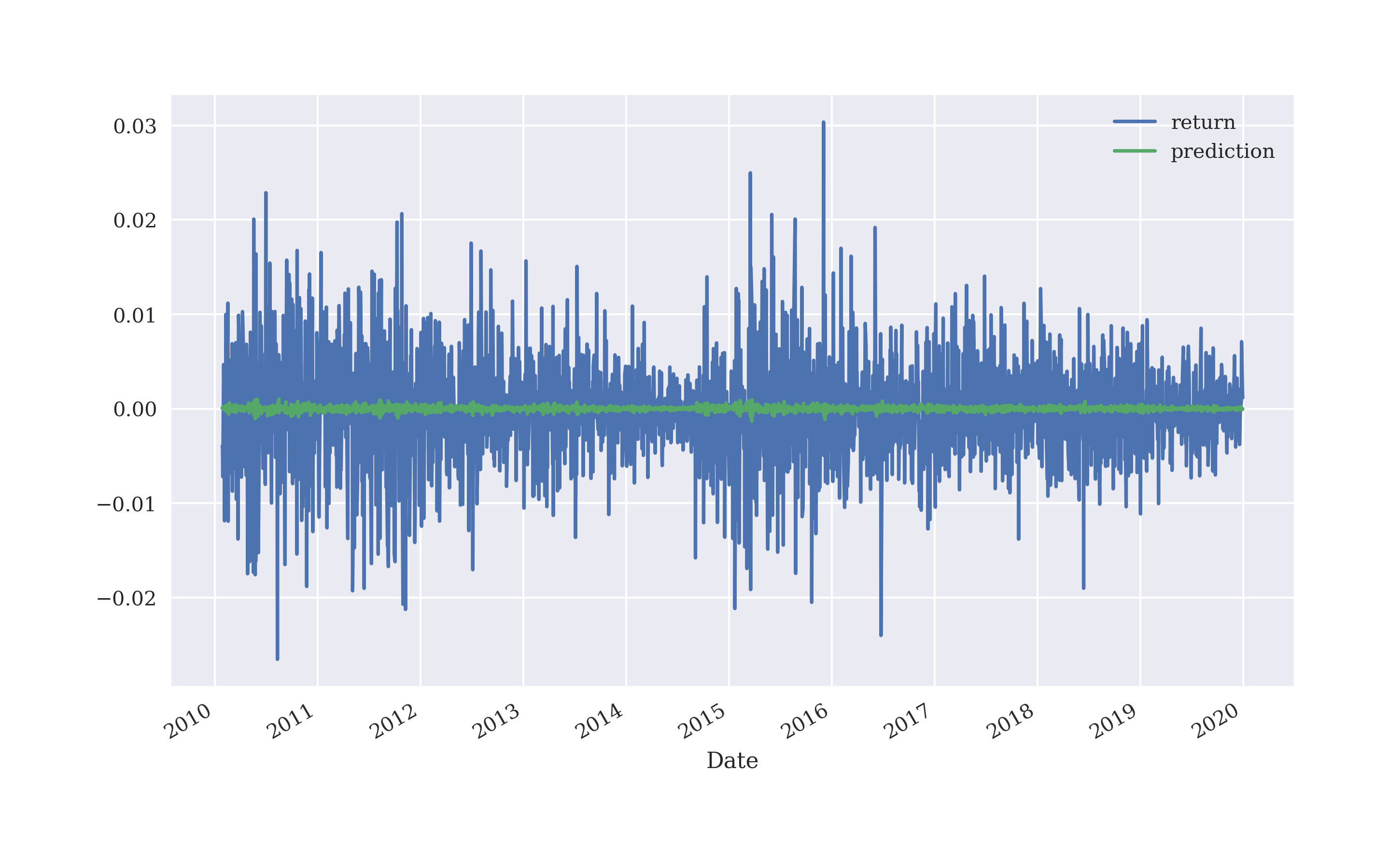
Figure 5-5. EUR/USD log returns and predicted values based on linear regression (5 lags)
From a trading point of view, one might argue that the magnitude of the forecasted return is not that relevant but rather whether the direction is forecasted correctly or not. To this end, a simple calculation yields an overview. Whenever the linear regression gets the direction right, meaning that the sign of the forecasted return is correct, the product of the market return and the predicted return is positive and otherwise negative. In the example case, the prediction is 1,250 times correct and 1,242 wrong which translates into a hit ratio of about 49.9% or almost exactly 50%.
In[38]:hits=np.sign(data['return']*data['prediction']).value_counts()In[39]:hitsOut[39]:1.01250-1.012420.013dtype:int64In[40]:hits.values[0]/sum(hits)Out[40]:0.499001996007984
Calculates the product of the market and predicted return, takes the sign of the results and counts the values.
Prints out the counts for the two possible values.
Calculates the hit ratio defined as the number of correct predictions given all predictions.
Predicting Future Market Direction
The question that arises is whether one can improve on the hit ratio by directly implementing the linear regression based on the sign of the log returns that serve as the dependent variable values. In theory at least, this simplifies the problem from predicting an absolute return value to the sign of the return value. The only change in the Python code to implement this reasoning is to use the sign values (that is 1.0 or -1.0 in Python) for the regression step. This indeed increases the number of hits to 1,301 and the hit ratio to about 51.9% — an improvement of 2 percentage points.
In[41]:reg=np.linalg.lstsq(data[cols],np.sign(data['return']),rcond=None)[0]In[42]:regOut[42]:array([-5.11938725,-2.24077248,-5.13080606,-3.03753232,-2.14819119])In[43]:data['prediction']=np.sign(np.dot(data[cols],reg))In[44]:data['prediction'].value_counts()Out[44]:1.01300-1.01205Name:prediction,dtype:int64In[45]:hits=np.sign(data['return']*data['prediction']).value_counts()In[46]:hitsOut[46]:1.01301-1.011910.013dtype:int64In[47]:hits.values[0]/sum(hits)Out[47]:0.5193612774451097
This takes the sign of the to be predicted return directly.
Also for the prediction step, only the sign is relevant.
Vectorized Backtesting of Regression-based Strategy
The hit ratio alone does not tell too much about the economic potential of a trading strategy using linear regression in the way presented so far. It is well known that the ten best and worst days in the markets for a given period of time considerably influence the overall performance of investments.2 In an ideal world, a long-short trader would try, of course, to benefit from both best and worst days by going long and short, respectively, on the basis of appropriate market timing indicators. Translated to the current context, this implies that in addition to the hit ratio the quality of the market timing matters too. Therefore, a backtesting along the lines of the approach in Chapter 4 can give a better picture of the value of regression for prediction.
Given the data that is already available, vectorized backtesting boils down to two lines of Python code including visualization. This is due to the fact that the prediction values already reflect the market positions (long or short). Figure 5-6 shows that the strategy under the current assumptions outperforms in-sample the market significantly (ignoring, among others, transaction costs).
In[48]:data.head()Out[48]:pricelag_1lag_2lag_3lag_4lag_5Date2010-01-201.4101-0.005858-0.008309-0.0005510.001103-0.0013102010-01-211.4090-0.013874-0.005858-0.008309-0.0005510.0011032010-01-221.4137-0.000780-0.013874-0.005858-0.008309-0.0005512010-01-251.41500.003330-0.000780-0.013874-0.005858-0.0083092010-01-261.40730.0009190.003330-0.000780-0.013874-0.005858predictionreturnDate2010-01-201.0-0.0138742010-01-211.0-0.0007802010-01-221.00.0033302010-01-251.00.0009192010-01-261.0-0.005457In[49]:data['strategy']=data['prediction']*data['return']In[50]:data[['return','strategy']].sum().apply(np.exp)Out[50]:return0.784026strategy1.654154dtype:float64In[51]:data[['return','strategy']].dropna().cumsum().apply(np.exp).plot(figsize=(10,6));
Multiplies the prediction values (positionings) by the market returns.
Calculates the gross performance of the base instrument and the strategy.
Plots the gross performance of the base instrument and the strategy over time (in-sample, no transaction costs).

Figure 5-6. Gross performance of EUR/USD and the regression-based strategy (5 lags)
Caution
The hit ratio of a prediction-based strategy is only one side of the coin when it gets to overall strategy performance. The other side is how well the strategy gets the market timing right. A strategy correctly predicting the best and worst days over a certain period of time might outperform the market even with a hit ratio below 50%. On the other hand, a strategy with a hit ratio well above 50% might still underperform the base instrument if it gets the rare, large movements wrong.
Generalizing the Approach
“Linear Regression Backtesting Class” presents a Python module containing a class for the vectorized backtesting of the regression-based trading strategy in the spirit of Chapter 4. In addition to allowing for an arbitrary amount to invest and proportional transaction costs, it also allows the in-sample fitting of the linear regression model and the out-of-sample evaluation. This means that the regression model is fitted based on one part of the data set, say for the years 2010 to 2015, and is evaluated based on another part of the data set, say for the years 2016 and 2019. For all strategies that involve an optimization or fitting step, this provides a more realistic view on the performance in practice since it helps avoiding the problems arising from data snooping and the overfitting of models (see also “Data Snooping and Overfitting”).
Figure 5-7 shows that the regression-based strategy based on five lags does outperform the EUR/USD base instrument for the particular configuration also out-of-sample and before accounting for transaction costs.
In[52]:importLRVectorBacktesterasLRIn[53]:lrbt=LR.LRVectorBacktester('EUR=','2010-1-1','2019-12-31',10000,0.0)In[54]:lrbt.run_strategy('2010-1-1','2019-12-31','2010-1-1','2019-12-31',lags=5)Out[54]:(17166.53,9442.42)In[55]:lrbt.run_strategy('2010-1-1','2017-12-31','2018-1-1','2019-12-31',lags=5)Out[55]:(10160.86,791.87)In[56]:lrbt.plot_results()
Imports the module as
LR.Instantiates an object of the
LRVectorBacktesterclass.Trains and evaluates the strategy on the same data set.
Uses two different data sets for the training and evaluation steps.
Plots the out-of-sample strategy performance compared to the market.
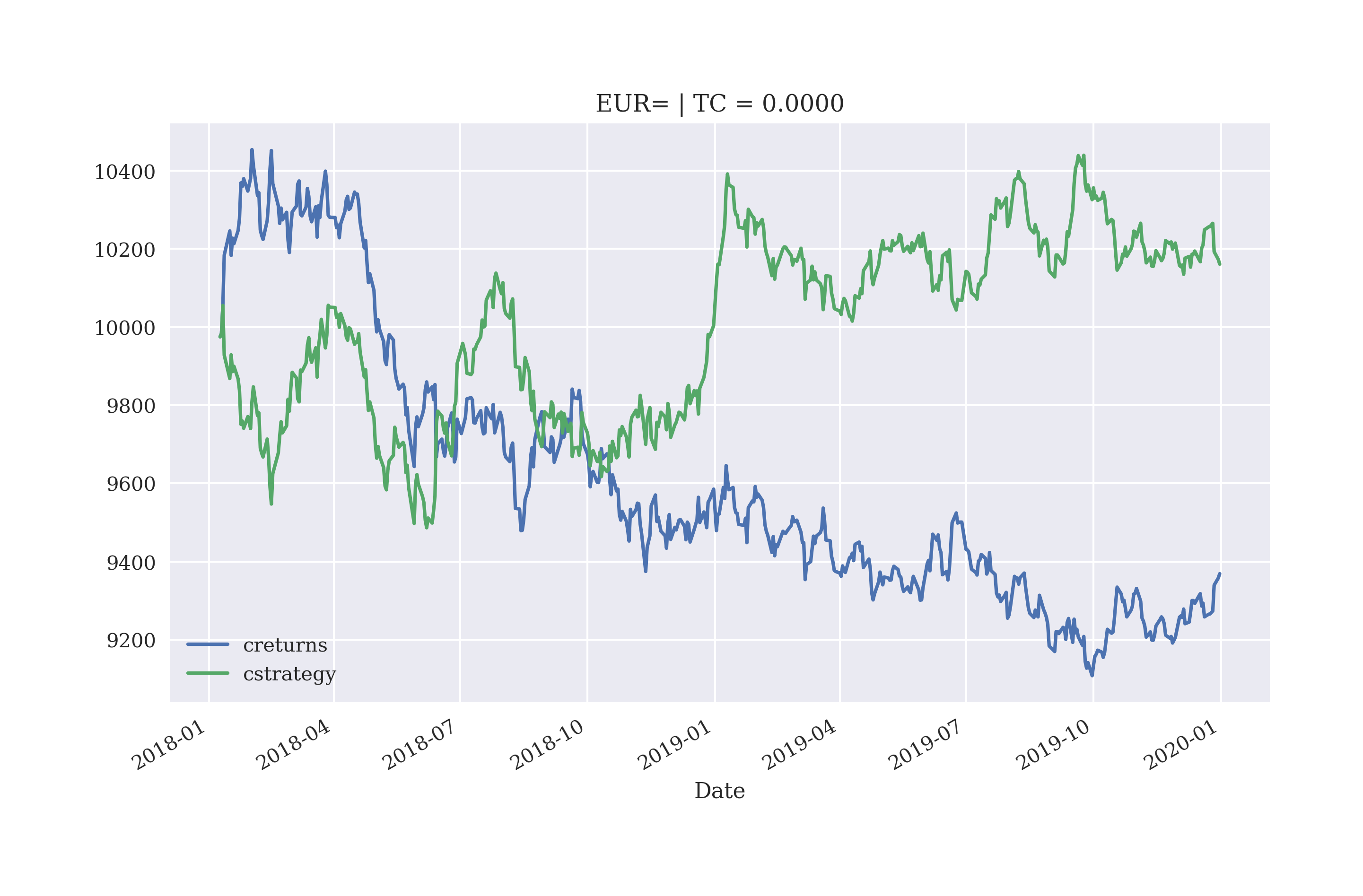
Figure 5-7. Gross performance of EUR/USD and the regression-based strategy (5 lags, out-of-sample, before transaction costs)
Consider the GDX ETF. The strategy configuration chosen shows an outperformance out-of-sample and after taking transaction costs into account (see Figure 5-8).
In[57]:lrbt=LR.LRVectorBacktester('GDX','2010-1-1','2019-12-31',10000,0.002)In[58]:lrbt.run_strategy('2010-1-1','2019-12-31','2010-1-1','2019-12-31',lags=7)Out[58]:(23642.32,17649.69)In[59]:lrbt.run_strategy('2010-1-1','2014-12-31','2015-1-1','2019-12-31',lags=7)Out[59]:(28513.35,14888.41)In[60]:lrbt.plot_results()
Changes to the time series data for
GDX.

Figure 5-8. Gross performance of the GDX ETF and the regression-based strategy (7 lags, out-of-sample, after transaction costs)
Using Machine Learning for Market Movement Prediction
Nowadays, the Python ecosystem provides a number of packages in the machine learning field. The most popular of these is scikit-learn (see scikit-learn home page), which is also one of the best documented and maintained packages. This section first introduces the API of the package based on linear regression, replicating some of the results of the previous section. It then goes on to use logistic regression as a classification algorithm to attack the problem of predicting the future market direction.
Linear Regression with scikit-learn
To introduce the scikit-learn API, revisiting the basic idea behind the prediction approach presented in this chapter is fruitful. Data preparation is the same as with NumPy only.
In[61]:x=np.arange(12)In[62]:xOut[62]:array([0,1,2,3,4,5,6,7,8,9,10,11])In[63]:lags=3In[64]:m=np.zeros((lags+1,len(x)-lags))In[65]:m[lags]=x[lags:]foriinrange(lags):m[i]=x[i:i-lags]
Using scikit-learn for our purposes mainly consists of three steps:
-
Model selection: A model is to be picked and instantiated.
-
Model fitting: The model is to be fitted to the data at hand.
-
Prediction: Given the fitted model, the prediction is conducted.
To apply linear regression, this translates into the following code that makes use of the linear_model sub-package for generalized linear models (see scikit-learn linear models page). By default, the LinearRegression model fits an intercept value.
In[66]:fromsklearnimportlinear_modelIn[67]:lm=linear_model.LinearRegression()In[68]:lm.fit(m[:lags].T,m[lags])Out[68]:LinearRegression()In[69]:lm.coef_Out[69]:array([0.33333333,0.33333333,0.33333333])In[70]:lm.intercept_Out[70]:2.0In[71]:lm.predict(m[:lags].T)Out[71]:array([3.,4.,5.,6.,7.,8.,9.,10.,11.])
Imports the generalized linear model classes.
Instantiates a linear regression model.
Fits the model to the data.
Prints out the optimal regression parameters.
Prints out the intercept values
Predicts the sought after values given the fitted model.
Setting the parameter fit_intercept to False, gives the exact same regression results as with NumPy and polyfit().
In[72]:lm=linear_model.LinearRegression(fit_intercept=False)In[73]:lm.fit(m[:lags].T,m[lags])Out[73]:LinearRegression(fit_intercept=False)In[74]:lm.coef_Out[74]:array([-0.66666667,0.33333333,1.33333333])In[75]:lm.intercept_Out[75]:0.0In[76]:lm.predict(m[:lags].T)Out[76]:array([3.,4.,5.,6.,7.,8.,9.,10.,11.])
This forces a fit without intercept value.
This example already illustrates quite well how to apply scikit-learn to the prediction problem. Due to its consistent API design, the basic approach carries over to other models as well.
A Simple Classification Problem
In a classification problem, it is to be decided to which of a limited set of categories (“classes”) a new observation belongs. A classical problem studied in machine learning is the identification of hand-written digits from 0 to 9. Such an identification leads to a correct result, say 3. Or it leads to a wrong result, say 6 or 8, where all such wrong results are equally wrong. In a financial market context, predicting the price of a financial instrument can lead to a numerical result that is far off the correct one or that is quite close to it. Predicting tomorrow’s market direction, there can only be a correct or a (“completely”) wrong result. The latter is a classification problem with the set of categories limited to, for example, “up” and “down” or “+1” and “-1” or “1” and “0" — by contrast, the former problem is an estimation problem.
A simple example for a classification problem is found on Wikipedia under Logistic Regression. The data set relates the number of hours studied to prepare for an exam by a number of students to the success of each student in passing the exam or not. While the number of hours studied is a real number (float object), the passing of the exam is either True or False — that is 1 or 0 in numbers. Figure 5-9 shows the data graphically.
In[77]:hours=np.array([0.5,0.75,1.,1.25,1.5,1.75,1.75,2.,2.25,2.5,2.75,3.,3.25,3.5,4.,4.25,4.5,4.75,5.,5.5])In[78]:success=np.array([0,0,0,0,0,0,1,0,1,0,1,0,1,0,1,1,1,1,1,1])In[79]:plt.figure(figsize=(10,6))plt.plot(hours,success,'ro')plt.ylim(-0.2,1.2);
The number of hours studied by the different students (sequence matters).
The success of each student in passing the exam (sequence matters).
Plots the data set taking
hoursasxvalues andsuccessasyvalues.Adjusts the limits of the
yaxis.
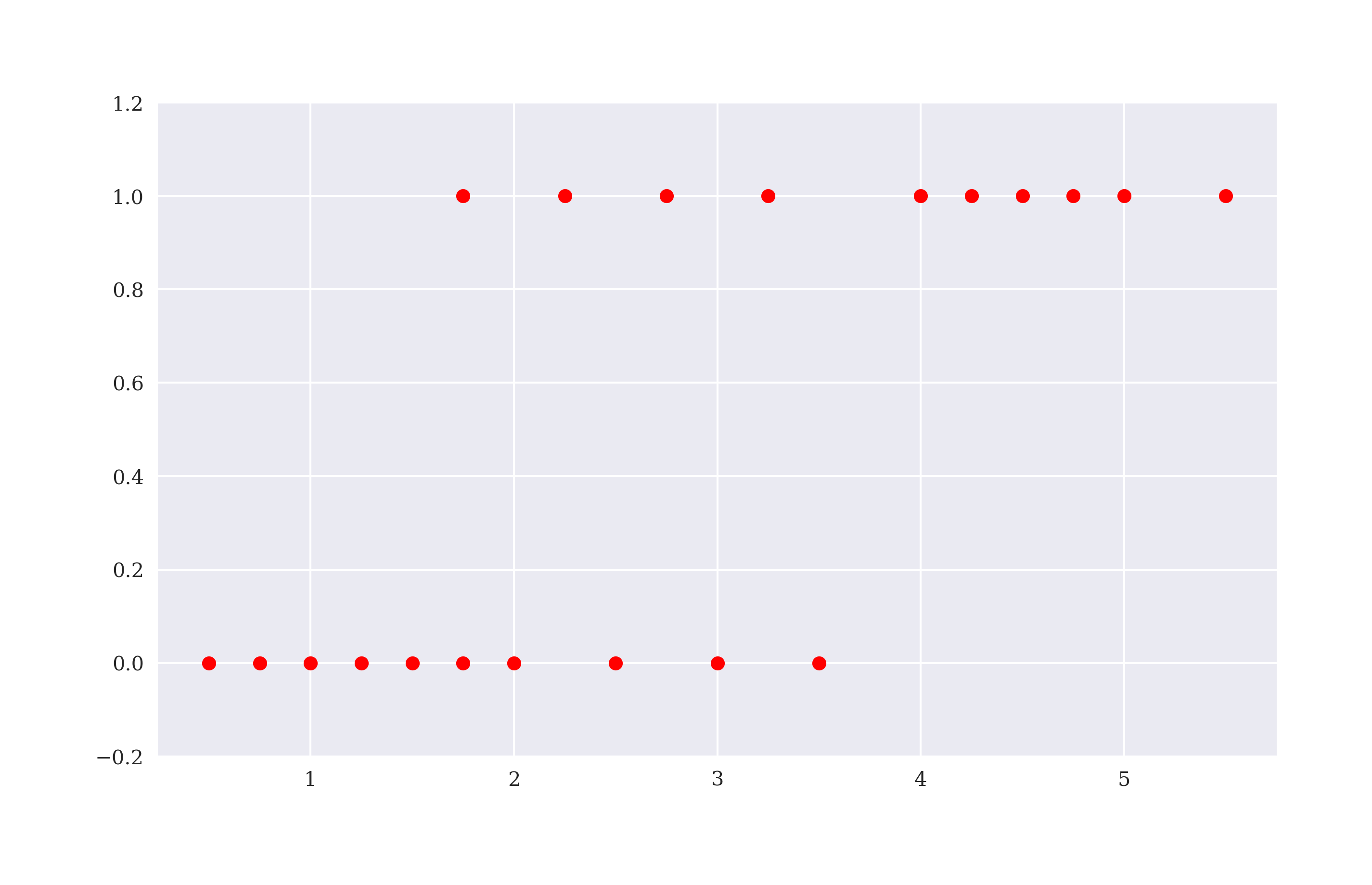
Figure 5-9. Example data for classification problem
The basic question typically raised in a such a context is: Given a certain number of hours studied by a student (not in the data set), will he/she pass the exam or not? What answer could linear regression give? Probably not one that is satisfying as Figure 5-10 shows. Given different numbers of hours studied, linear regression gives (prediction) values mainly between 0 and 1 but also lower and higher. But there can only be failure or success as the outcome of taking the exam.
In[80]:reg=np.polyfit(hours,success,deg=1)In[81]:plt.figure(figsize=(10,6))plt.plot(hours,success,'ro')plt.plot(hours,np.polyval(reg,hours),'b')plt.ylim(-0.2,1.2);
Implements a linear regression on the data set.
Plots the regression line in addition to the data set.

Figure 5-10. Linear regression applied to classification problem
This is where classification algorithms, like logistic regression and support vector machines, come into play. For illustration, the application of logistic regression suffices (see James et al. (2013, ch. 4) for more background information). The respective class is also found in the linear_model sub-package. Figure 5-11 shows the result of the following Python code. This time, there is a clear cut (prediction) value for every different input value. Between 0 and 2 hours the model predicts that a students fails. For all values equal or higher than 2.75 hours, the model predicts that a student passes the exam.
In[82]:lm=linear_model.LogisticRegression(solver='lbfgs')In[83]:hrs=hours.reshape(1,-1).TIn[84]:lm.fit(hrs,success)Out[84]:LogisticRegression()In[85]:prediction=lm.predict(hrs)In[86]:plt.figure(figsize=(10,6))plt.plot(hours,success,'ro',label='data')plt.plot(hours,prediction,'b',label='prediction')plt.legend(loc=0)plt.ylim(-0.2,1.2);
Instantiates the logistic regression model.
Reshapes the one-dimensional
ndarrayobject to a two-dimensional one (required byscikit-learn).Implements the fitting step.
Implements the prediction step given the fitted model.

Figure 5-11. Logistic regression applied to classification problem
However, as Figure 5-11 shows there is no guarantee that 2.75 hours or more lead to success. It is just “more probable” to succeed from that many hours on than to fail. This probabilistic reasoning can be analyzed and visualized as well based on the same model instance as the following code illustrates. The dashed line in Figure 5-12 shows the probability for succeeding (monotonically increasing). The dash-dotted line shows it for failing (monotonically decreasing).
In[87]:prob=lm.predict_proba(hrs)In[88]:plt.figure(figsize=(10,6))plt.plot(hours,success,'ro')plt.plot(hours,prediction,'b')plt.plot(hours,prob.T[0],'m--',label='$p(h)$ for zero')plt.plot(hours,prob.T[1],'g-.',label='$p(h)$ for one')plt.ylim(-0.2,1.2)plt.legend(loc=0);
Predicts probabilities for succeeding and failing, respectively.
Plots the probabilities for failing.
Plots the probabilities for succeeding.

Figure 5-12. Probabilities for succeeding and failing, respectively, based on logistic regression
Tip
scikit-learn does a good job in providing access to a great variety of machine learning models in a unified way. The examples show that the API for applying logistic regression does not differ from the one for linear regression. scikit-learn therefore is well suited to test a number of appropriate machine learning models in a certain application scenario without altering the Python code that much.
Equipped with the basics, the next step is to apply logistic regression to the problem of predicting market direction.
Using Logistic Regression to Predict Market Direction
In machine learning, one generally speaks of features instead of independent or explanatory variables as in a regression context. The simple classification example has a single feature only: the number of hours studied. In practice, one often has more than one feature that can be used for classification. Given the prediction approach introduced in this chapter, one can identify a feature by a lag. Therefore, working with three lags from the time series data means that there are three features. As possible outcomes or categories, there are only +1 and -1 for an upwards and a downwards movement, respectively. Although the wording changes, the formalism stays the same, in particular with regard to deriving the matrix, now called the feature matrix.
The following code presents an alternative to creating a pandas DataFrame based “feature matrix” to which the three step procedure applies equally well — if not in a more Pythonic fashion. The feature matrix now is a sub-set of the columns in the original data set.
In[89]:symbol='GLD'In[90]:data=pd.DataFrame(raw[symbol])In[91]:data.rename(columns={symbol:'price'},inplace=True)In[92]:data['return']=np.log(data['price']/data['price'].shift(1))In[93]:data.dropna(inplace=True)In[94]:lags=3In[95]:cols=[]forlaginrange(1,lags+1):col='lag_{}'.format(lag)data[col]=data['return'].shift(lag)cols.append(col)In[96]:data.dropna(inplace=True)
Instantiates an empty
listobject to collect column names.Creates a
strobject for the column name.Adds a new column to the
DataFrameobject with the respective lag data.Appends the column name to the
listobject.Makes sure that the data set is complete.
Logistic regression improves the hit ratio compared to linear regression by more than a percentage point to about 54.5%. Figure 5-13 shows the performance of the strategy based on logistic regression-based predictions. Although the hit ratio is higher, the performance is worse than with linear regression.
In[97]:fromsklearn.metricsimportaccuracy_scoreIn[98]:lm=linear_model.LogisticRegression(C=1e7,solver='lbfgs',multi_class='auto',max_iter=1000)In[99]:lm.fit(data[cols],np.sign(data['return']))Out[99]:LogisticRegression(C=10000000.0,max_iter=1000)In[100]:data['prediction']=lm.predict(data[cols])In[101]:data['prediction'].value_counts()Out[101]:1.01983-1.0529Name:prediction,dtype:int64In[102]:hits=np.sign(data['return'].iloc[lags:]*data['prediction'].iloc[lags:]).value_counts()In[103]:hitsOut[103]:1.01338-1.011590.012dtype:int64In[104]:accuracy_score(data['prediction'],np.sign(data['return']))Out[104]:0.5338375796178344In[105]:data['strategy']=data['prediction']*data['return']In[106]:data[['return','strategy']].sum().apply(np.exp)Out[106]:return1.289478strategy2.458716dtype:float64In[107]:data[['return','strategy']].cumsum().apply(np.exp).plot(figsize=(10,6));
Instantiates the model object using a
Cvalue that gives less weight to the regularization term (see Generalized Linear Models page).Fits the model based on the sign of the returns to be predicted.
Generates a new column in the
DataFrameobject and writes the prediction values to it.Shows the number of the resulting long and short positions, respectively.
Calculates the number of correct and wrong predictions.
The accuracy (hit ratio) is 53.3% in this case.
However, the gross performance of the strategy …
… is much higher when compared the passive benchmark investment.
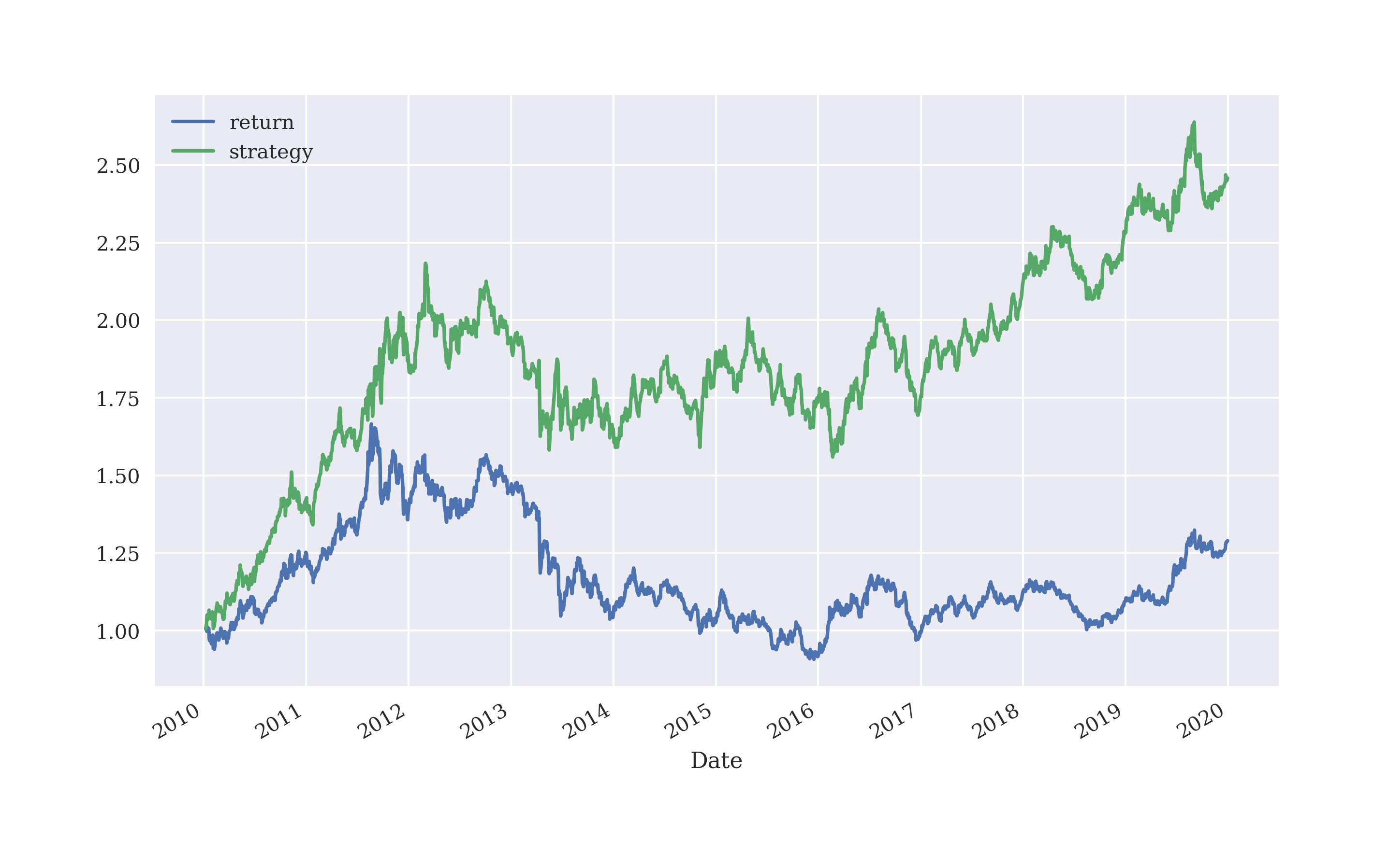
Figure 5-13. Gross performance of GLD ETF and logistic regression-based strategy (3 lags, in-sample)
Increasing the number of lags used from 3 to 5 decreases the hit ratio but improves the gross performance of the strategy to some extent (in-sample, before transaction costs). Figure 5-14 shows the resulting performance.
In[108]:data=pd.DataFrame(raw[symbol])In[109]:data.rename(columns={symbol:'price'},inplace=True)In[110]:data['return']=np.log(data['price']/data['price'].shift(1))In[111]:lags=5In[112]:cols=[]forlaginrange(1,lags+1):col='lag_%d'%lagdata[col]=data['price'].shift(lag)cols.append(col)In[113]:data.dropna(inplace=True)In[114]:lm.fit(data[cols],np.sign(data['return']))Out[114]:LogisticRegression(C=10000000.0,max_iter=1000)In[115]:data['prediction']=lm.predict(data[cols])In[116]:data['prediction'].value_counts()Out[116]:1.02047-1.0464Name:prediction,dtype:int64In[117]:hits=np.sign(data['return'].iloc[lags:]*data['prediction'].iloc[lags:]).value_counts()In[118]:hitsOut[118]:1.01331-1.011630.012dtype:int64In[119]:accuracy_score(data['prediction'],np.sign(data['return']))Out[119]:0.5312624452409399In[120]:data['strategy']=data['prediction']*data['return']In[121]:data[['return','strategy']].sum().apply(np.exp)Out[121]:return1.283110strategy2.656833dtype:float64In[122]:data[['return','strategy']].cumsum().apply(np.exp).plot(figsize=(10,6));
Increases the number of lags to 5.
Fits the model based on 5 lags.
There are now significantly more short positions with the new parametrization.
The accuracy (hit ratio) decreases to 53.1%.
The cumulative performance also increases significantly.
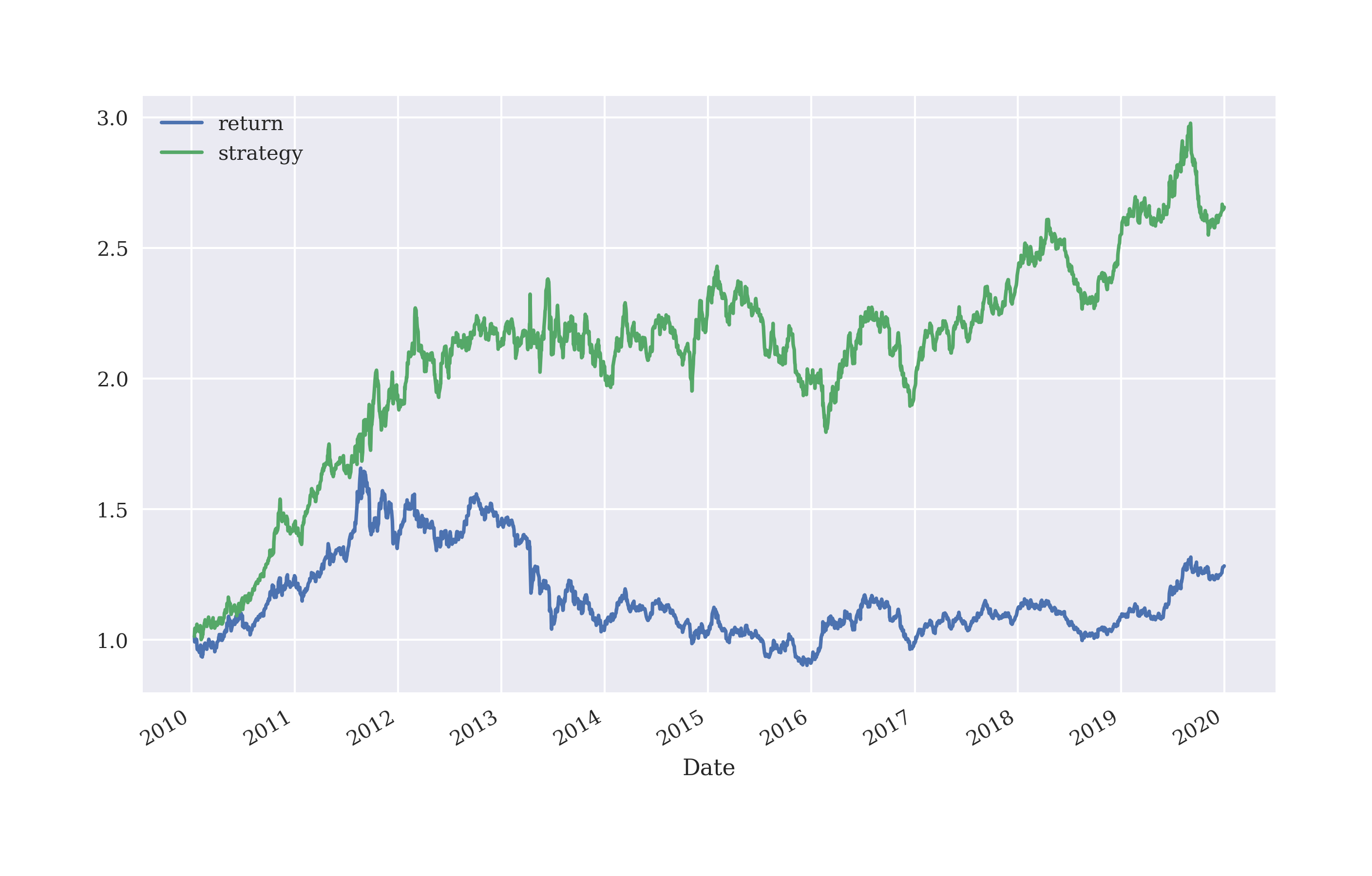
Figure 5-14. Gross performance of GLD ETF and logistic regression-based strategy (5 lags, in-sample)
Caution
You have to be careful with not falling into the overfitting trap here. A more realistic picture is obtained by an approach that uses training data (= in-sample data) for the fitting of the model and test data (= out-of-sample data) for the evaluation of the strategy performance. This is done in the following when the approach is generalized again in the form of a Python class.
Generalizing the Approach
“Classification Algorithm Backtesting Class” presents a Python module with a class for the vectorized backtesting of strategies based on linear models from scikit-learn. Although only linear and logistic regression are implemented, the number of models is easily increased. In principle, the ScikitVectorBacktester class could inherit selected methods from the LRVectorBacktester but it is presented in a self-contained fashion. This makes it easier to enhance and re-use this class for practical applications.
Based on the ScikitBacktesterClass, an out-of-sample evaluation of the logistic regression-based strategy is possible. The example uses the EUR/USD exchange rate as the base instrument. Figure 5-15 illustrates that the strategy outperforms the base instrument during the out-of-sample period (spanning the year 2019) — this, however, without considering transaction costs as before.
In[123]:importScikitVectorBacktesterasSCIIn[124]:scibt=SCI.ScikitVectorBacktester('EUR=','2010-1-1','2019-12-31',10000,0.0,'logistic')In[125]:scibt.run_strategy('2015-1-1','2019-12-31','2015-1-1','2019-12-31',lags=15)Out[125]:(12192.18,2189.5)In[126]:scibt.run_strategy('2016-1-1','2018-12-31','2019-1-1','2019-12-31',lags=15)Out[126]:(10580.54,729.93)In[127]:scibt.plot_results()

Figure 5-15. Cumulative returns of S&P 500 and out-of-sample logistic regression-based strategy (15 lags, no transaction costs)
As another example, consider the same strategy applied to the GDX ETF, for which an out-of-sample outperformance (over the year 2018) is shown Figure 5-16 (before transaction costs).
In[128]:scibt=SCI.ScikitVectorBacktester('GDX','2010-1-1','2019-12-31',10000,0.00,'logistic')In[129]:scibt.run_strategy('2013-1-1','2017-12-31','2018-1-1','2018-12-31',lags=10)Out[129]:(12686.81,4032.73)In[130]:scibt.plot_results()
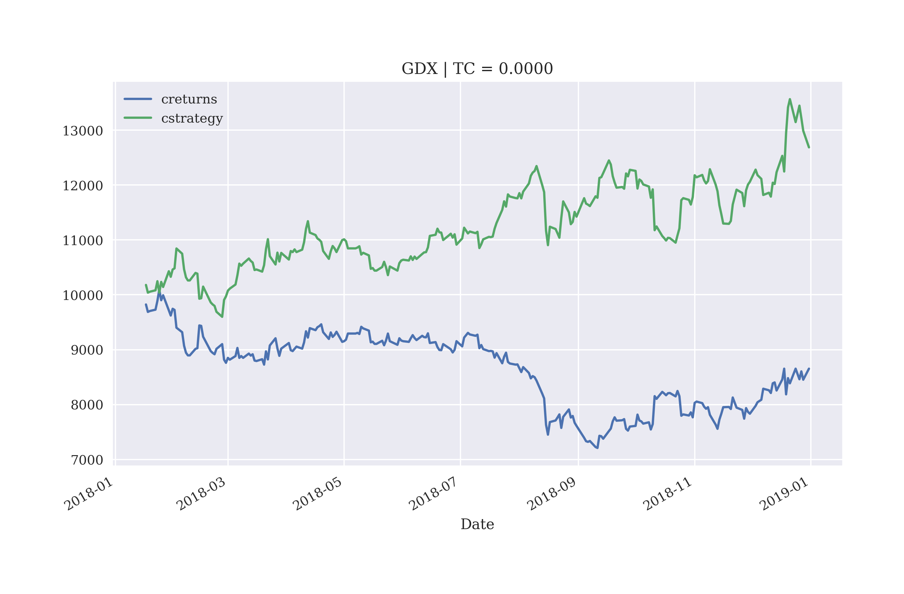
Figure 5-16. Gross performance of GDX ETF and logistic regression-based strategy (10 lags, out-of-sample, no transaction costs)
Figure 5-17 shows how the gross performance is diminished — leading even to a net loss — when taking transaction costs into account, while keeping all other parameters constant.
In[131]:scibt=SCI.ScikitVectorBacktester('GDX','2010-1-1','2019-12-31',10000,0.0025,'logistic')In[132]:scibt.run_strategy('2013-1-1','2017-12-31','2018-1-1','2018-12-31',lags=10)Out[132]:(9588.48,934.4)In[133]:scibt.plot_results()
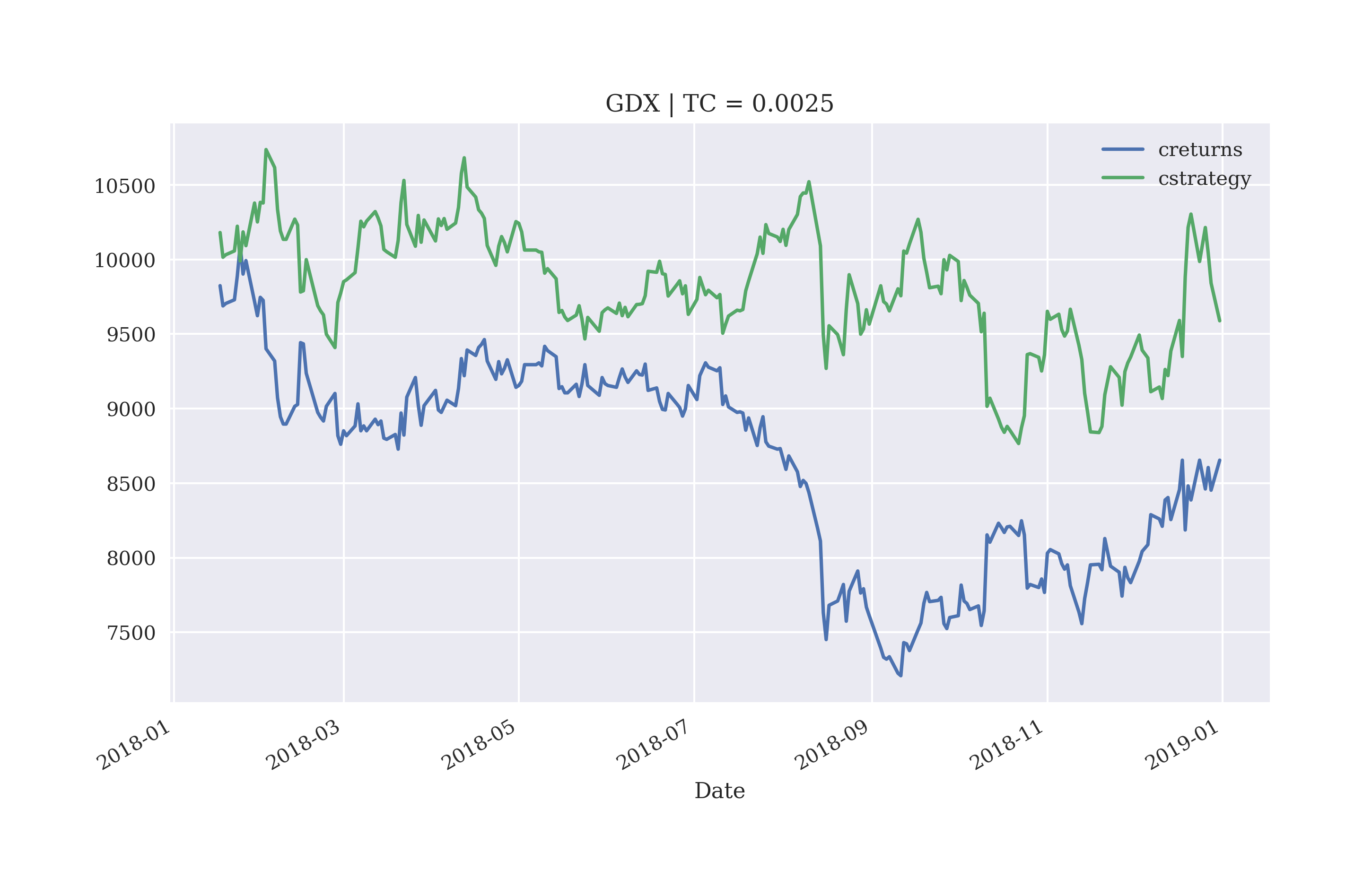
Figure 5-17. Gross performance of GDX ETF and logistic regression-based strategy (10 lags, out-of-sample, with transaction costs)
Caution
Applying sophisticated machine learning techniques to stock market prediction often yields promising results early on. In several examples, the strategies backtested outperform the base instrument significantly in-sample. Quite often, such stellar performances are due to a mix of simplifying assumptions and also due to an overfitting of the prediction model. For example, testing the very same strategy instead of in-sample on a out-of-sample data set and adding transaction costs — as two ways of getting to a more realistic picture — often shows that the performance of the considered strategy “suddenly” trails the base instrument performance-wise or turns to a net loss.
Using Deep Learning for Market Movement Prediction
Right from the open sourcing and publication by Google, the deep learning library TensorFlow has attracted much interest and wide-spread application. This section applies TensorFlow in the same way as the previous one scikit-learn to the prediction of stock market movements modeled as a classification problem. However, TensorFlow is not used directly, it is rather used via the evenly popular Keras deep learning package. Keras can be thought of as providing a higher level abstraction to the TensorFlow package with a more easy to understand and use API. The libraries are best installed via pip install tensorflow and pip install keras. scikit-learn also offers classes to apply neural networks to classification problems.
For more background information on deep learning and Keras see the books by Goodfellow et al. (2016) and Chollet (2017), respectively.
The Simple Classification Problem Revisited
To illustrate the basic approach of applying neural networks to classification problems, the simple classification problem introduced in the previous section proves again useful.
In[134]:hours=np.array([0.5,0.75,1.,1.25,1.5,1.75,1.75,2.,2.25,2.5,2.75,3.,3.25,3.5,4.,4.25,4.5,4.75,5.,5.5])In[135]:success=np.array([0,0,0,0,0,0,1,0,1,0,1,0,1,0,1,1,1,1,1,1])In[136]:data=pd.DataFrame({'hours':hours,'success':success})In[137]:data.info()<class'pandas.core.frame.DataFrame'>RangeIndex:20entries,0to19Datacolumns(total2columns):# Column Non-Null Count Dtype----------------------------0hours20non-nullfloat641success20non-nullint64dtypes:float64(1),int64(1)memoryusage:448.0bytes
Stores the two data sub-sets in a
DataFrameobject.Prints out the meta information for the
DataFrameobject.
With these preparations, MLPClassifier from scikit-learn can be imported and straightforwardly applied.3 “MLP” in this context stands for multi-layer perceptron which is another expression for dense neural network. As before, the API to apply neural networks with scikit-learn is basically the same.
In[138]:fromsklearn.neural_networkimportMLPClassifierIn[139]:model=MLPClassifier(hidden_layer_sizes=[32],max_iter=1000,random_state=100)
Import the
MLPClassifierobject fromscikit-learn.Instantiates the
MLPClassifierobject.
The code below fits the model, generates the predictions and plots the results as shown in Figure 5-18.
In[140]:model.fit(data['hours'].values.reshape(-1,1),data['success'])Out[140]:MLPClassifier(hidden_layer_sizes=[32],max_iter=1000,random_state=100)In[141]:data['prediction']=model.predict(data['hours'].values.reshape(-1,1))In[142]:data.tail()Out[142]:hourssuccessprediction154.2511164.5011174.7511185.0011195.5011In[143]:data.plot(x='hours',y=['success','prediction'],style=['ro','b-'],ylim=[-.1,1.1],figsize=(10,6));
Fits the neural network for classification.
Generates the prediction values based on the fitted model.
Plots the original data and the prediction values.

Figure 5-18. Base data and prediction results with MLPClassifier for the simple classification example
The simple example shows that the application of the deep learning approach is quite similar to the approach with scikit-learn and the LogisticRegression model object — the API is basically the same, only the parameters are different.
Using Deep Neural Networks to Predict Market Direction
The next step is to apply the approach to stock market data in the form of log returns from a financial time series. First, the data needs to be retrieved and prepared.
In[144]:symbol='EUR='In[145]:data=pd.DataFrame(raw[symbol])In[146]:data.rename(columns={symbol:'price'},inplace=True)In[147]:data['return']=np.log(data['price']/data['price'].shift(1))In[148]:data['direction']=np.where(data['return']>0,1,0)In[149]:lags=5In[150]:cols=[]forlaginrange(1,lags+1):col=f'lag_{lag}'data[col]=data['return'].shift(lag)cols.append(col)data.dropna(inplace=True)In[151]:data.round(4).tail()Out[151]:pricereturndirectionlag_1lag_2lag_3lag_4lag_5Date2019-12-241.10870.000110.0007-0.00380.0008-0.00340.00062019-12-261.10960.000810.00010.0007-0.00380.0008-0.00342019-12-271.11750.007110.00080.00010.0007-0.00380.00082019-12-301.11970.002010.00710.00080.00010.0007-0.00382019-12-311.12100.001210.00200.00710.00080.00010.0007
Reads the data from the
CSVfile.Picks the single time series column of interest.
Renames the only column to
price.Calculates the log returns and defines the
directionas a binary column.Creates the lagged data.
Creates new
DataFramecolumns with the log returns shifted by the respective number of lags.Deletes rows containing
NaNvalues.Prints out the final five rows indicating the “patterns” emerging in the five feature columns.
The code below uses a dense neural network (DNN) with the Keras package4, defines training and test data sub-sets, defines the feature columns and labels and fits the classifier. In the backend, Keras uses the TensorFlow package to accomplish the task. Figure 5-19 shows how the accuracy of the DNN classifier changes for both the training and validation data sets during training. As validation data set, 20% of the training data (without shuffling) is used.
In[152]:importtensorflowastffromkeras.modelsimportSequentialfromkeras.layersimportDensefromkeras.optimizersimportAdam,RMSpropIn[153]:optimizer=Adam(learning_rate=0.0001)In[154]:defset_seeds(seed=100):random.seed(seed)np.random.seed(seed)tf.random.set_seed(100)In[155]:set_seeds()model=Sequential()model.add(Dense(64,activation='relu',input_shape=(lags,)))model.add(Dense(64,activation='relu'))model.add(Dense(1,activation='sigmoid'))model.compile(optimizer=optimizer,loss='binary_crossentropy',metrics=['accuracy'])In[156]:cutoff='2017-12-31'In[157]:training_data=data[data.index<cutoff].copy()In[158]:mu,std=training_data.mean(),training_data.std()In[159]:training_data_=(training_data-mu)/stdIn[160]:test_data=data[data.index>=cutoff].copy()In[161]:test_data_=(test_data-mu)/stdIn[162]:%%timemodel.fit(training_data[cols],training_data['direction'],epochs=50,verbose=False,validation_split=0.2,shuffle=False)CPUtimes:user4.86s,sys:989ms,total:5.85sWalltime:3.34sOut[162]:<tensorflow.python.keras.callbacks.Historyat0x7f996a0a2880>In[163]:res=pd.DataFrame(model.history.history)In[164]:res[['accuracy','val_accuracy']].plot(figsize=(10,6),style='--');
Imports the
TensorFlowpackageImports the required model object from
Keras.Imports the relevant layer object from
Keras.A
Sequentialmodel is instantiated.The hidden layers and the output layer are defined.
Compiles the
Sequentialmodel object for classification.Defines the cutoff date between the training and test data.
Defines the training and test data sets
Normalizes the features data by Gaussian normalization.
Fits the model to the training data set.
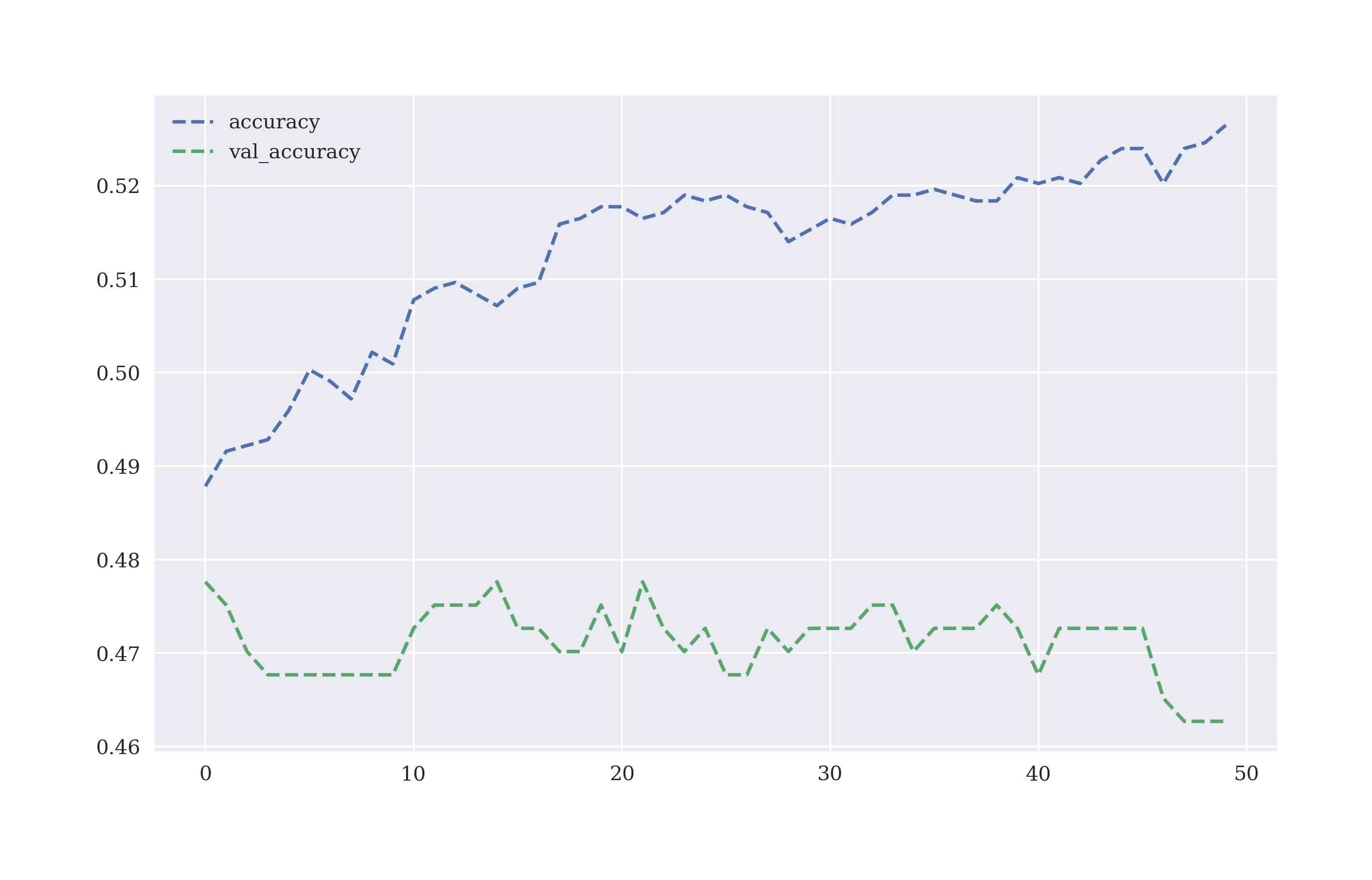
Figure 5-19. Accuracy of DNN classifier on training and validation data per training step
Equipped with the fitted classifier, the model can generate predictions on the training data set. Figure 5-20 shows the strategy gross performance compared to the base instrument (in-sample).
In[165]:model.evaluate(training_data_[cols],training_data['direction'])63/63[==============================]-0s586us/step-loss:0.7556-accuracy:0.5152Out[165]:[0.7555528879165649,0.5151968002319336]In[166]:pred=np.where(model.predict_classes(training_data_[cols])>0.5,1,0)WARNING:tensorflow:From<ipython-input-166-2827c9e13527>:1:Sequential.predict_classes(fromtensorflow.python.keras.engine.sequential)isdeprecatedandwillberemovedafter2021-01-01.Instructionsforupdating:Pleaseuseinstead:*`np.argmax(model.predict(x), axis=-1)`,ifyourmodeldoesmulti-classclassification(e.g.ifitusesa`softmax`last-layeractivation).*`(model.predict(x) > 0.5).astype("int32")`,ifyourmodeldoesbinaryclassification(e.g.ifitusesa`sigmoid`last-layeractivation).In[167]:pred[:30].flatten()Out[167]:array([0,0,0,0,0,1,1,1,1,0,0,0,1,1,1,0,0,0,1,1,0,0,0,1,0,1,0,1,0,0])In[168]:training_data['prediction']=np.where(pred>0,1,-1)In[169]:training_data['strategy']=(training_data['prediction']*training_data['return'])In[170]:training_data[['return','strategy']].sum().apply(np.exp)Out[170]:return0.826569strategy1.317303dtype:float64In[171]:training_data[['return','strategy']].cumsum().apply(np.exp).plot(figsize=(10,6));
Predicts the market direction in-sample.
Transforms the predictions into long-short positions,
+1, -1.Calculates the strategy returns given the positions.
Plots and compares the strategy performance to the benchmark performance (in-sample).
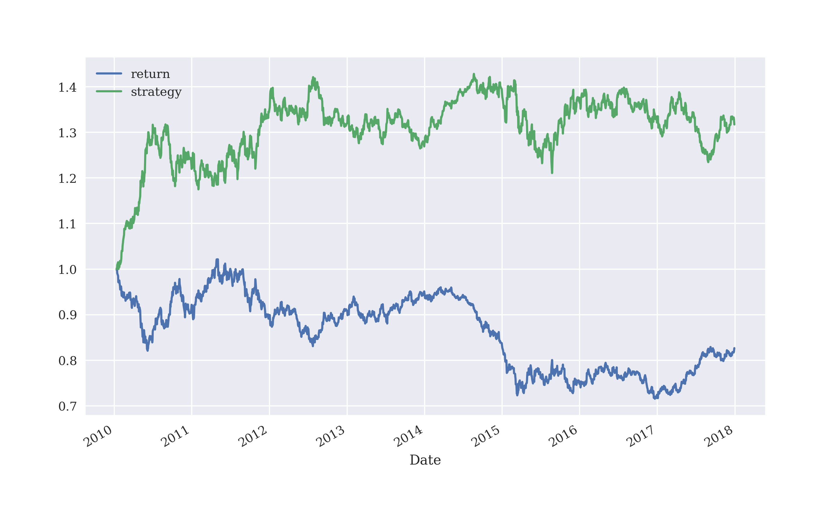
Figure 5-20. Gross performance of EUR/USD compared deep learning-based strategy (in-sample, no transaction costs)
The strategy seems to perform somewhat better than the base instrument on the training data set (in-sample, without transaction costs). However, the more interesting question is how it performs on the test data set (out-of-sample). After a wobbly start, the strategy also outperforms the base instrument out-of-sample as Figure 5-21 illustrates. This is despite the fact that the accuracy of the classifier is below 50% on the test data set.
In[172]:model.evaluate(test_data_[cols],test_data['direction'])16/16[==============================]-0s676us/step-loss:0.7292-accuracy:0.5050Out[172]:[0.7292129993438721,0.5049701929092407]In[173]:pred=np.where(model.predict(test_data_[cols])>0.5,1,0)In[174]:test_data['prediction']=np.where(pred>0,1,-1)In[175]:test_data['prediction'].value_counts()Out[175]:-13681135Name:prediction,dtype:int64In[176]:test_data['strategy']=(test_data['prediction']*test_data['return'])In[177]:test_data[['return','strategy']].sum().apply(np.exp)Out[177]:return0.934478strategy1.109065dtype:float64In[178]:test_data[['return','strategy']].cumsum().apply(np.exp).plot(figsize=(10,6));

Figure 5-21. Gross performance of EUR/USD compared to deep learning-based strategy (out-of-sample, no transaction costs)
Adding Different Types of Features
So far, the analysis mainly focuses on the log returns directly. It is, of course, possible to not only add more classes/categories but to also add other types of features to the mix, like, for example, ones based momentum, volatility, or distance measures. The code that follows derives the additional features and adds them to the data set.
In[179]:data['momentum']=data['return'].rolling(5).mean().shift(1)In[180]:data['volatility']=data['return'].rolling(20).std().shift(1)In[181]:data['distance']=(data['price']-data['price'].rolling(50).mean()).shift(1)In[182]:data.dropna(inplace=True)In[183]:cols.extend(['momentum','volatility','distance'])In[184]:(data.round(4).tail())pricereturndirectionlag_1lag_2lag_3lag_4lag_5Date2019-12-241.10870.000110.0007-0.00380.0008-0.00340.00062019-12-261.10960.000810.00010.0007-0.00380.0008-0.00342019-12-271.11750.007110.00080.00010.0007-0.00380.00082019-12-301.11970.002010.00710.00080.00010.0007-0.00382019-12-311.12100.001210.00200.00710.00080.00010.0007momentumvolatilitydistanceDate2019-12-24-0.00100.00240.00052019-12-26-0.00110.00240.00042019-12-27-0.00030.00240.00122019-12-300.00100.00280.00892019-12-310.00210.00280.0110
The momentum-based feature.
The volatility-based feature.
The distance-based feature.
The next step is to redefine the training and test data sets, to normalize the features data and to update the model to reflect the new features columns.
In[185]:training_data=data[data.index<cutoff].copy()In[186]:mu,std=training_data.mean(),training_data.std()In[187]:training_data_=(training_data-mu)/stdIn[188]:test_data=data[data.index>=cutoff].copy()In[189]:test_data_=(test_data-mu)/stdIn[190]:set_seeds()model=Sequential()model.add(Dense(32,activation='relu',input_shape=(len(cols),)))model.add(Dense(32,activation='relu'))model.add(Dense(1,activation='sigmoid'))model.compile(optimizer=optimizer,loss='binary_crossentropy',metrics=['accuracy'])
The
input_shapeparameter is adjusted to reflect the new number of features.
Based on the enriched feature set, the classifier can be trained. The in-sample performance of the strategy is quite a bit better than before as illustrated in Figure 5-22.
In[191]:%%timemodel.fit(training_data_[cols],training_data['direction'],verbose=False,epochs=25)CPUtimes:user2.32s,sys:577ms,total:2.9sWalltime:1.48sOut[191]:<tensorflow.python.keras.callbacks.Historyat0x7f996d35c100>In[192]:model.evaluate(training_data_[cols],training_data['direction'])62/62[==============================]-0s649us/step-loss:0.6816-accuracy:0.5646Out[192]:[0.6816270351409912,0.5646397471427917]In[193]:pred=np.where(model.predict(training_data_[cols])>0.5,1,0)In[194]:training_data['prediction']=np.where(pred>0,1,-1)In[195]:training_data['strategy']=(training_data['prediction']*training_data['return'])In[196]:training_data[['return','strategy']].sum().apply(np.exp)Out[196]:return0.901074strategy2.703377dtype:float64In[197]:training_data[['return','strategy']].cumsum().apply(np.exp).plot(figsize=(10,6));
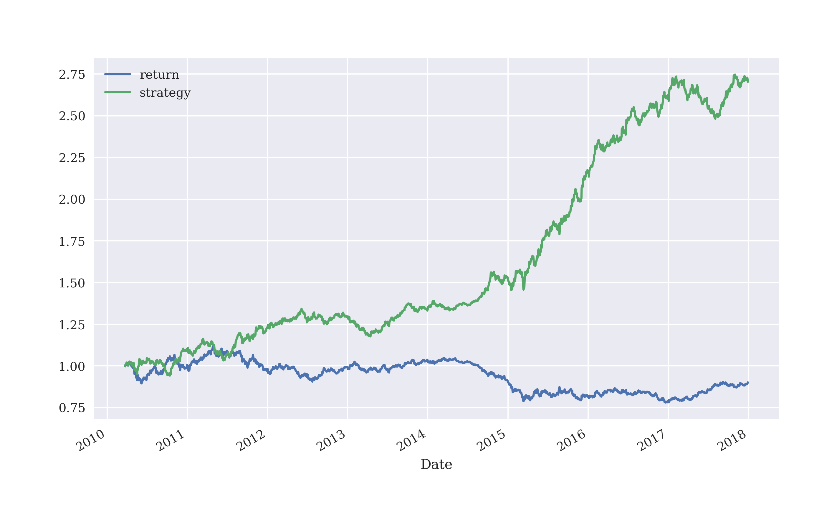
Figure 5-22. Gross performance of EUR/USD compared to deep learning-based strategy (in-sample, additional features)
The final step is the evaluation of the classifier and the derivation of the strategy performance out-of-sample. The classifier performs also significantly better, ceteris paribus, when compared to the case without the additional features. As before, the start is a bit (see Figure 5-23).
In[198]:model.evaluate(test_data_[cols],test_data['direction'])16/16[==============================]-0s800us/step-loss:0.6931-accuracy:0.5507Out[198]:[0.6931276321411133,0.5506958365440369]In[199]:pred=np.where(model.predict(test_data_[cols])>0.5,1,0)In[200]:test_data['prediction']=np.where(pred>0,1,-1)In[201]:test_data['prediction'].value_counts()Out[201]:-13351168Name:prediction,dtype:int64In[202]:test_data['strategy']=(test_data['prediction']*test_data['return'])In[203]:test_data[['return','strategy']].sum().apply(np.exp)Out[203]:return0.934478strategy1.144385dtype:float64In[204]:test_data[['return','strategy']].cumsum().apply(np.exp).plot(figsize=(10,6));

Figure 5-23. Gross performance of EUR/USD compared to deep learning-based strategy (out-of-sample, additional features)
The Keras package in combination with the TensorFlow package as its backend allows to make use of the most recent advances in deep learning — like for instance deep neural network (DNN) classifiers — for algorithmic trading. The application is as straightforward as applying other machine learning models with scikit-learn. The approach illustrated in this section allows for an easy enhancement with regard to the (different types of) features used.
Tip
As an exercise, it is worthwhile to code a Python class (in the spirit of “Linear Regression Backtesting Class” and “Classification Algorithm Backtesting Class”) that allows for a more systematic and realistic usage of the Keras package for financial market prediction and the backtesting of respective trading strategies.
Conclusions
Predicting future market movements is the holy grail in finance. It means to find the truth. It means to overcome efficient markets. If one can do it with a considerable edge, then stellar investment and trading returns are the consequence. This chapter introduces statistical techniques — from the fields of traditional statistics, machine learning, and deep learning — to predict the future market direction based on past returns or similar financial quantities. Some first in-sample results are promising, both for linear as well as logistic regression. However, a more reliable impression is gained when evaluating such strategies out-of-sample and also when factoring in transaction costs.
This chapter does not claim to have found the holy grail. It rather offers a glimpse on techniques that could prove useful in the search for it. The unified API of scikit-learn also makes it easy to replace, for example, one linear model by another one. In that sense, the ScikitBacktesterClass can be used as a starting point to explore more machine learning models and to apply them to financial time series prediction.
The quote at the beginning of the chapter from the Terminator 2 movie from 1991 is rather optimistic with regard to how fast and what exactly computers might be able to learn and acquire consciousness. No matter if you believe that computers will replace human beings in most areas of life or not or if they one day become indeed self-aware, they have proven useful to human beings as supporting devices in almost any area of life. And algorithms like those used in machine learning, deep learning, or artificial intelligence hold at least the promise to let them even become better algorithmic traders in the near future. A more detailed account of these topics and considerations if found in Hilpisch (2020).
Further Resources
The books by Guido and Müller (2016) and VanderPlas (2016) provide practical introductions to machine learning with Python and scikit-learn. The book by Hilpisch (2020) focuses exclusively on the application of algorithms for machine and deep learning to the problem of identifying statistical inefficiencies and exploiting economic inefficiencies through algorithmic trading.
-
Guido, Sarah and Andreas Müller (2016): Introduction to Machine Learning with Python — A Guide for Data Scientists. O’Reilly, Hoboken et al.
-
Hilpisch, Yves (2020): Artificial Intelligence in Finance — A Python-based Guide. O’Reilly, Beijing et al.
-
VanderPlas, Jake (2016): Python Data Science Handbook — Essential Tools for Working with Data. O’Reilly, Beijing et al.
The books by Hastie et al. (2008) and James et al. (2013) provide a thorough, mathematical overview of popular machine learning techniques and algorithms.
-
Hastie, Trevor, Robert Tibshirani and Jerome Friedman (2008): The Elements of Statistical Learning. 2nd ed., Springer, New York et al.
-
James, Gareth James, Daniela Witten, Trevor Hastie and Robert Tibshirani (2013): Introduction to Statistical Learning. Springer, New York et al.
For more background information on deep learning and Keras, refer to these books:
-
Chollet, Francois (2017): Deep Learning with Python. Manning, Shelter Island.
-
Goodfellow, Ian, Yoshua Bengio and Aaron Courville (2016): Deep Learning. MIT Press, Cambridge, http://deeplearningbook.org.
Python Scripts
This section presents Python scripts referenced and used in this chapter.
Linear Regression Backtesting Class
The following presents Python code with a class for the vectorized backtesting of strategies based on linear regression used for the prediction of the direction of market movements.
## Python Module with Class# for Vectorized Backtesting# of Linear Regression-based Strategies## Python for Algorithmic Trading# (c) Dr. Yves J. Hilpisch# The Python Quants GmbH#importnumpyasnpimportpandasaspdclassLRVectorBacktester(object):''' Class for the vectorized backtesting ofLinear Regression-based trading strategies.Attributes==========symbol: strTR RIC (financial instrument) to work withstart: strstart date for data selectionend: strend date for data selectionamount: int, floatamount to be invested at the beginningtc: floatproportional transaction costs (e.g. 0.5% = 0.005) per tradeMethods=======get_data:retrieves and prepares the base data setselect_data:selects a sub-set of the dataprepare_lags:prepares the lagged data for the regressionfit_model:implements the regression steprun_strategy:runs the backtest for the regression-based strategyplot_results:plots the performance of the strategy compared to the symbol'''def__init__(self,symbol,start,end,amount,tc):self.symbol=symbolself.start=startself.end=endself.amount=amountself.tc=tcself.results=Noneself.get_data()defget_data(self):''' Retrieves and prepares the data.'''raw=pd.read_csv('http://hilpisch.com/pyalgo_eikon_eod_data.csv',index_col=0,parse_dates=True).dropna()raw=pd.DataFrame(raw[self.symbol])raw=raw.loc[self.start:self.end]raw.rename(columns={self.symbol:'price'},inplace=True)raw['returns']=np.log(raw/raw.shift(1))self.data=raw.dropna()defselect_data(self,start,end):''' Selects sub-sets of the financial data.'''data=self.data[(self.data.index>=start)&(self.data.index<=end)].copy()returndatadefprepare_lags(self,start,end):''' Prepares the lagged data for the regression and prediction steps.'''data=self.select_data(start,end)self.cols=[]forlaginrange(1,self.lags+1):col=f'lag_{lag}'data[col]=data['returns'].shift(lag)self.cols.append(col)data.dropna(inplace=True)self.lagged_data=datadeffit_model(self,start,end):''' Implements the regression step.'''self.prepare_lags(start,end)reg=np.linalg.lstsq(self.lagged_data[self.cols],np.sign(self.lagged_data['returns']),rcond=None)[0]self.reg=regdefrun_strategy(self,start_in,end_in,start_out,end_out,lags=3):''' Backtests the trading strategy.'''self.lags=lagsself.fit_model(start_in,end_in)self.results=self.select_data(start_out,end_out).iloc[lags:]self.prepare_lags(start_out,end_out)prediction=np.sign(np.dot(self.lagged_data[self.cols],self.reg))self.results['prediction']=predictionself.results['strategy']=self.results['prediction']*self.results['returns']# determine when a trade takes placetrades=self.results['prediction'].diff().fillna(0)!=0# subtract transaction costs from return when trade takes placeself.results['strategy'][trades]-=self.tcself.results['creturns']=self.amount*self.results['returns'].cumsum().apply(np.exp)self.results['cstrategy']=self.amount*self.results['strategy'].cumsum().apply(np.exp)# gross performance of the strategyaperf=self.results['cstrategy'].iloc[-1]# out-/underperformance of strategyoperf=aperf-self.results['creturns'].iloc[-1]returnround(aperf,2),round(operf,2)defplot_results(self):''' Plots the cumulative performance of the trading strategycompared to the symbol.'''ifself.resultsisNone:('No results to plot yet. Run a strategy.')title='%s| TC =%.4f'%(self.symbol,self.tc)self.results[['creturns','cstrategy']].plot(title=title,figsize=(10,6))if__name__=='__main__':lrbt=LRVectorBacktester('.SPX','2010-1-1','2018-06-29',10000,0.0)(lrbt.run_strategy('2010-1-1','2019-12-31','2010-1-1','2019-12-31'))(lrbt.run_strategy('2010-1-1','2015-12-31','2016-1-1','2019-12-31'))lrbt=LRVectorBacktester('GDX','2010-1-1','2019-12-31',10000,0.001)(lrbt.run_strategy('2010-1-1','2019-12-31','2010-1-1','2019-12-31',lags=5))(lrbt.run_strategy('2010-1-1','2016-12-31','2017-1-1','2019-12-31',lags=5))
Classification Algorithm Backtesting Class
The following presents Python code with a class for the vectorized backtesting of strategies based on logistic regression, as a standard classification algorithm, used for the prediction of the direction of market movements.
## Python Module with Class# for Vectorized Backtesting# of Machine Learning-based Strategies## Python for Algorithmic Trading# (c) Dr. Yves J. Hilpisch# The Python Quants GmbH#importnumpyasnpimportpandasaspdfromsklearnimportlinear_modelclassScikitVectorBacktester(object):''' Class for the vectorized backtesting ofMachine Learning-based trading strategies.Attributes==========symbol: strTR RIC (financial instrument) to work withstart: strstart date for data selectionend: strend date for data selectionamount: int, floatamount to be invested at the beginningtc: floatproportional transaction costs (e.g. 0.5% = 0.005) per trademodel: streither 'regression' or 'logistic'Methods=======get_data:retrieves and prepares the base data setselect_data:selects a sub-set of the dataprepare_features:prepares the features data for the model fittingfit_model:implements the fitting steprun_strategy:runs the backtest for the regression-based strategyplot_results:plots the performance of the strategy compared to the symbol'''def__init__(self,symbol,start,end,amount,tc,model):self.symbol=symbolself.start=startself.end=endself.amount=amountself.tc=tcself.results=Noneifmodel=='regression':self.model=linear_model.LinearRegression()elifmodel=='logistic':self.model=linear_model.LogisticRegression(C=1e6,solver='lbfgs',multi_class='ovr',max_iter=1000)else:raiseValueError('Model not known or not yet implemented.')self.get_data()defget_data(self):''' Retrieves and prepares the data.'''raw=pd.read_csv('http://hilpisch.com/pyalgo_eikon_eod_data.csv',index_col=0,parse_dates=True).dropna()raw=pd.DataFrame(raw[self.symbol])raw=raw.loc[self.start:self.end]raw.rename(columns={self.symbol:'price'},inplace=True)raw['returns']=np.log(raw/raw.shift(1))self.data=raw.dropna()defselect_data(self,start,end):''' Selects sub-sets of the financial data.'''data=self.data[(self.data.index>=start)&(self.data.index<=end)].copy()returndatadefprepare_features(self,start,end):''' Prepares the feature columns for the regression and prediction steps.'''self.data_subset=self.select_data(start,end)self.feature_columns=[]forlaginrange(1,self.lags+1):col='lag_{}'.format(lag)self.data_subset[col]=self.data_subset['returns'].shift(lag)self.feature_columns.append(col)self.data_subset.dropna(inplace=True)deffit_model(self,start,end):''' Implements the fitting step.'''self.prepare_features(start,end)self.model.fit(self.data_subset[self.feature_columns],np.sign(self.data_subset['returns']))defrun_strategy(self,start_in,end_in,start_out,end_out,lags=3):''' Backtests the trading strategy.'''self.lags=lagsself.fit_model(start_in,end_in)# data = self.select_data(start_out, end_out)self.prepare_features(start_out,end_out)prediction=self.model.predict(self.data_subset[self.feature_columns])self.data_subset['prediction']=predictionself.data_subset['strategy']=(self.data_subset['prediction']*self.data_subset['returns'])# determine when a trade takes placetrades=self.data_subset['prediction'].diff().fillna(0)!=0# subtract transaction costs from return when trade takes placeself.data_subset['strategy'][trades]-=self.tcself.data_subset['creturns']=(self.amount*self.data_subset['returns'].cumsum().apply(np.exp))self.data_subset['cstrategy']=(self.amount*self.data_subset['strategy'].cumsum().apply(np.exp))self.results=self.data_subset# absolute performance of the strategyaperf=self.results['cstrategy'].iloc[-1]# out-/underperformance of strategyoperf=aperf-self.results['creturns'].iloc[-1]returnround(aperf,2),round(operf,2)defplot_results(self):''' Plots the cumulative performance of the trading strategycompared to the symbol.'''ifself.resultsisNone:('No results to plot yet. Run a strategy.')title='%s| TC =%.4f'%(self.symbol,self.tc)self.results[['creturns','cstrategy']].plot(title=title,figsize=(10,6))if__name__=='__main__':scibt=ScikitVectorBacktester('.SPX','2010-1-1','2019-12-31',10000,0.0,'regression')(scibt.run_strategy('2010-1-1','2019-12-31','2010-1-1','2019-12-31'))(scibt.run_strategy('2010-1-1','2016-12-31','2017-1-1','2019-12-31'))scibt=ScikitVectorBacktester('.SPX','2010-1-1','2019-12-31',10000,0.0,'logistic')(scibt.run_strategy('2010-1-1','2019-12-31','2010-1-1','2019-12-31'))(scibt.run_strategy('2010-1-1','2016-12-31','2017-1-1','2019-12-31'))scibt=ScikitVectorBacktester('.SPX','2010-1-1','2019-12-31',10000,0.001,'logistic')(scibt.run_strategy('2010-1-1','2019-12-31','2010-1-1','2019-12-31',lags=15))(scibt.run_strategy('2010-1-1','2013-12-31','2014-1-1','2019-12-31',lags=15))
1 The books by Guido and Müller (2016) and VanderPlas (2016) provide practical, general introductions to machine learning with Python.
2 See, for example, the discussion in Invesco (2016): “The Tale of 10 Days”.
3 For details, see https://scikit-learn.org/stable/modules/generated/sklearn.neural_network.MLPClassifier.html.
4 For details, refer to https://keras.io/layers/core/.