
9
The VPLS Case Study
In the previous chapters of this book, the main focus has been the analysis of the QOS tools, one by one, and in Chapter 3 we focused on the challenges of a QOS deployment. We have now introduced all the different parts of the QOS equation and are ready to move forward and present three case studies that illustrate end-to-end QOS deployments in the format of case studies. The case study in this chapter focuses on a Virtual Private LAN Service (VPLS) scenario, the second one is focused in the internals of a Data Center, and the third one in a mobile network. The reason for selecting these three realms is due to the fact that they are the most challenging ones at present, but unquestionably the lessons learned from it can be translated to other less complex realms, like an enterprise deployment by just removing the MPLS component out of the equation of this case study. Using these case studies, we glue together the QOS concepts and tools we have discussed and also explain how to cope with some of the challenges highlighted in Chapter 3. However, as previously discussed, any QOS deployment is never completely independent of other network components, such as the network routing characteristics, because, for example, routing can place constraints on the number of hops, or which particular hops, are crossed by the traffic. So it is not accurate to present a QOS case study without first analyzing the network and its characteristics. However, discussion of the other network components is limited only to what is strictly necessary so that the focus of the case studies always remains on QOS.
This chapter starts by presenting an overview of the network technologies being used and how the particular services are implemented. Then we define the service specifications, starting off with some loose constraints that we discuss and tune as the case study evolves. Finally, we discuss which QOS tools should be used and how they should be tuned to achieve the desired end result. This is illustrated by following a packet as it traverses across the network.
9.1 High-Level Case Study Overview
Before discussing the specific details of this case study, it will be helpful to provide a high-level perspective of its design and components. This case study focuses on a service provider network that offers VPN services to its customers. For several years, VPN services have provided the highest revenue for service providers, and when it comes to Layer 2 services, VPLS is one of the most popular ones being commonly used, not just by the service providers but also for Data Center interconnections. For a service provider network, one primary reason is that VPLS is implemented with MPLS tunnels, also referred to as label-switched paths (LSPs), as illustrated in Figure 9.1.

Figure 9.1 MPLS tunnels used to forward the customer traffic
These tunnels carry the VPLS traffic (shown as white packets in Figure 9.1) between the routers on which the service end points are located. So the QOS deployment interacts with MPLS, and so must be tailored to take advantage of the range of MPLS features. Control traffic, represented in Figure 9.1 as black triangles, is what keeps the network alive and breathing. This traffic is crucial, because without it, for example, the MPLS tunnels used by customer traffic to travel between the service end points cannot be established. VPLS is the support used for the services.
In this case study, the customer has different classes of service from which to choose. Here, the network has four classes of service: real time (RT), business (BU), data (DA), and best effort (BE). We explain later in this chapter how these classes differ. Looking at traffic flow, when customer traffic arrives at the network, it is split into a maximum of four classes of service, as illustrated in Figure 9.2.

Figure 9.2 Customer traffic
From the network perspective, traffic arriving from the customer has no class of service assigned to it, so the first task performed by the edge router is to split the customer traffic into the different classes of service. This split is made according to the agreement established between the customer and the service provider network at the service end point. Then, based on the service connectivity rules, traffic is placed inside one or more LSPs toward the remote service end points.
Figure 9.2 shows two major groups of traffic inside the network, customer and control traffic, and the customer traffic can be split into four subgroups: RT, BU, DA, and BE. A key difference between customer and control traffic is that the customer traffic transits the network, that is, it has a source and destination external to the network, while control traffic exists only within the network.
This overview of the network internals and the service offered is our starting point. As the case study evolves, we will introduce different technologies and different types of traffic. Let us now focus on each network component individually.
9.2 Virtual Private Networks
In a nutshell, virtual private networks (VPNs) provide connectivity to customers that have sites geographically spread across one or more cities, or even countries, sparing the customers from having to invest in their own infrastructure to establish connectivity between its sites.
However, this connectivity carries the “Private” keyword attached to it, so the customer traffic must be kept private. This has several implications for routing, security, and other network technologies. For QOS, this requirement implies that the customer traffic must be delivered between sites based on a set of parameters defined and agreed upon by both parties, independently of any other traffic that may be present inside the service provider’s network. This set of parameters is usually defined in a service-level agreement (SLA). To meet the SLA, the customer traffic exchanged between its several sites is placed into one or more classes of service, and for each one, a set of parameters is defined that must be met. For example, one parameter may be the maximum delay inserted into the transmission of traffic as it travels from customer site X1 to X2, an example illustrated in Figure 9.3.

Figure 9.3 Delay assurance across a service provider network
The VPN service has two variants, Layer 3 (L3) and Layer 2 (L2). To a certain degree, the popularity of MPLS as a technology owes much to the simplicity it offers for service providers implementing VPNs. The success of L2VPNs is closely linked to the Ethernet boom as a transport technology (because its cost is lower than other transmission mediums) and also to the fact that L2VPNs do not need a routing protocol running between the customer device and the service provider’s PE router. So the PE router does not play a role in the routing of customer traffic. One result is that the customer device can be a switch or a server that does not necessarily support routing functionality.
9.3 Service Overview
The service implemented using VPLS operates as a hub-and-spoke VLAN, and the network customer-facing interfaces are all Ethernet.
A hub site can be seen as a central aggregation or traffic distribution point, and spoke sites as transmitters (or receivers) toward the hub site, as illustrated in Figure 9.4.

Figure 9.4 Hub-and-spoke VLAN
In terms of connectivity, a hub site can communicate with multiple spoke sites or with other hub sites if they exist, but a spoke site can communicate only with a single hub site. These connectivity rules mean that for Layer 2 forwarding, there is no need for MAC learning or resolution at the spoke sites, because all that traffic that is transmitted (or received) has only one possible destination (or source), the hub site.
There are several applicable scenarios for this type of service. One example is a hub site that contains multiple financial services servers that wish to distribute information to multiple customers in wholesale fashion, meaning that the customers have no connectivity with each other. Another example is Digital Subscriber Line (DSL) traffic aggregation, in which multiple Digital Subscriber Line Access Multiplexers (DSLAMs) aggregating DSL traffic connect to the hub points, and the hub-and-spoke VLAN carry that traffic toward a BRAS router located at a spoke point. This scenario can be expanded further by including a backup BRAS router at a secondary spoke point, to act, in case the primary router fails, as illustrated in Figure 9.5.

Figure 9.5 DSL scenario for the hub-and-spoke VLAN
Hub points may or may not be able to communicate directly with each other. Typically, inter-DSLAM communication must be done via the BRAS router to apply accounting tools and to enforce connectivity rules. This means that “local switching” between hubs may need to be blocked.
The fact that no MAC learning is done at the spoke sites is a benefit for scaling, but it raises the question of how the BRAS router can select a specific DSLAM to which to send traffic. Typically, DSLAM selection is achieved by configuring different Ethernet VLAN tags on the hub interfaces facing the DSLAMs. For example, the Ethernet interface (either logical or physical) that faces DSLAM #3 at the hub point can be configured with an outer VLAN tag of 100 and an inner tag of 300, as illustrated in Figure 9.6.
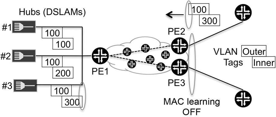
Figure 9.6 Packet forwarding inside the hub-and-spoke VLAN
If the primary BRAS wants to send traffic toward DSLAM #3, it must place these tags in the traffic it sends toward PE2, where the spoke point is located. PE2 forwards that traffic blindly (without any MAC address resolution) toward PE1, where the hub point is located. Then inside the hub point, the traffic is forwarded toward the Ethernet interface to which DSLAM #3 is connected. As a side note, although PE2 does not perform any MAC learning, MAC learning must be enabled on the BRAS itself.
9.4 Service Technical Implementation
The main technology in the L2VPN realm to implement the service described in the previous section is VPLS, in particular using its mesh-group functionality combined with Layer 2 Circuits (l2ckt).
Within a VPLS domain, the PE routers must be fully meshed at the data plane so a forwarding split-horizon rule can be applied. This rule means that if a PE router receives traffic from any other PE, it can forward it only to customer-facing interfaces but never to other PE routers. The VPLS protocol can be seen as transforming the network into one large and single Ethernet segment, so the existence of the forwarding split-horizon rule is necessary to ensure that there are no Layer 2 loops inside the network. This rule is the VPLS alternative to the Spanning Tree Protocols (STPs), which have been shown not to scale outside the LAN realm. The price to pay for the requirement of this full mesh between PE routers at the data plane is obviously scaling and complexity.
The mesh-group functionality breaks the VPLS behavior as a single Ethernet segment by dividing the VPLS domain into different mesh groups, where the obligation for a full mesh at the data plane between PE routers exists only within each mesh group. So traffic received from another PE in the same mesh group can indeed be forwarded to other PE routers, but only if they belong to a different mesh group. As a concept, mesh groups are not entirely new in the networking world, because they already exist in the routing realm.
Let us now demonstrate how this functionality can be used to provide the connectivity requirements desired for the hub-and-spoke VLAN.
As illustrated in Figure 9.7, a VPLS instance is created at PE1 containing two mesh groups, one name MESH-HUB and other MESH-SPOKES. The MESH-HUB group contains all the hub interfaces, and local switching between them can be blocked if required. The second mesh group, MESH-SPOKES, contains the spoke sites. It is from this mesh group that the two l2ckts, which terminate at PE2 and PE3, are created. Terminating the l2ckts inside the VPLS domain is the secret to not requiring any MAC learning at the spoke sites. L2ckts are often called pseudowires, because they emulate a wire across the network in the sense that any traffic injected at one end of the wire is received at the other end, so there is no need for any MAC resolution.
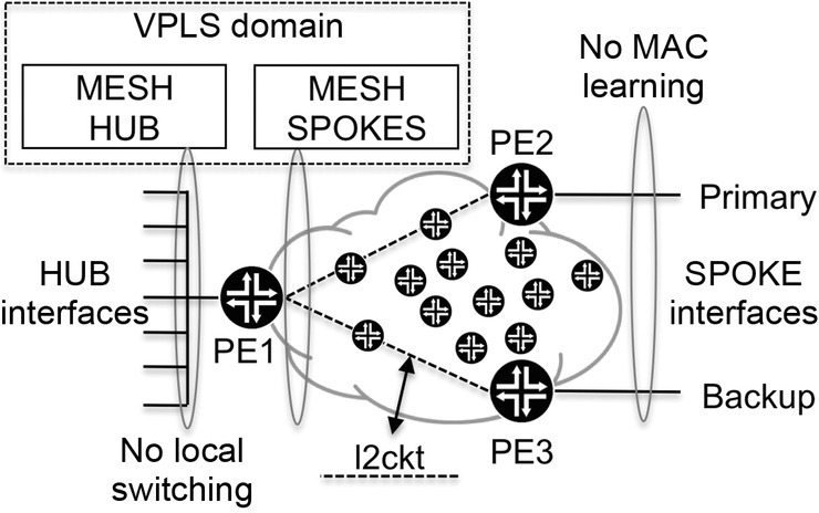
Figure 9.7 VPLS mesh groups
The topology shown in Figure 9.7 ensures resiliency since primary and secondary sites can be defined and also has the scaling gain that the spoke interfaces do not require any active MAC learning.
9.5 Network Internals
The previous sections have focused on the events that take place at the network edge. Now let us now turn our attention to the core of the network.
For routing, the network uses MPLS-TE with strict Explicit Routing Object (ERO), which allows 100% control over the path that traffic takes across the network, as illustrated in Figure 9.8.

Figure 9.8 Network internal routing with MPLS-TE ERO
Two distinct paths, a primary and a secondary, are always created between any two PE routers for redundancy. If a failure occurs on the primary path, the ingress node moves traffic onto the secondary path. However, to make things interesting, let us assume that each primary path crosses a maximum of four hops between the source and the destination, but for the secondary path that number increases to five. The importance of this difference with regard to QOS will become clearer later in this chapter, when we discuss the dimensioning of queue sizes.
While these sections have provided a high-level perspective of the network and services, a complete understanding requires additional knowledge about the MPLS, VPLS, and L2VPN realms. A reader seeking more information about these topics should refer to the links provided in the Further Reading section of this chapter. However, to discuss the QOS part of this case study, it is not crucial to understand all the VPLS mechanics but just simply to accept the connectivity rules mentioned earlier and the values of the maximum number of hops crossed by the primary and secondary paths.
Now that the service and networks basics have been presented, we can move on to the QOS section of this case study.
9.6 Classes of Service and Queue Mapping
A customer accesses the network by a VLAN that is subject to an aggregate rate, which establishes the maximum ingress and egress rates of customer traffic entering and leaving the network. Once the rate is defined, the customer divides it into four classes of service: real time (RT), business (BU), data (DA), and best effort (BE), whose characteristics are summarized in Table 9.1.
Table 9.1 Classes of service requirements
| COS | Traffic sensitivity | CIR/PIR | Admission control | ||
| Delay | Jitter | Packet loss | |||
| RT | Max 75 ms | High | High | Only CIR | |
| BU | Medium | Medium | High | Only CIR | Y |
| DA | Low | Both | |||
| BE | PIR | N | |||
The RT class of service is the most sensitive in terms of requirements, including an assurance that no more than 75 ms of delay be inserted into this traffic as it crosses the network between the service end points. As the reader can notice, the definition of the RT class of service is highly sensitive to jitter, but a maximum value is not defined. We discuss this more later in this case study.
The BU class of service is the second most sensitive in terms of requirements, although it is not as sensitive to delay and jitter as RT. However, it still has strict requirements regarding packet loss.
For the CIR/PIR model, the main interest lies in the DA class of service, because DA traffic will be split into green and yellow depending on its arrival rate.
In terms of admission control, an aggregate rate is applied to customer traffic as a whole as it enters the network, and then each class of service is subject to a specific rate. The only exception is BE traffic because this class has no CIR value, so no specific rate is applied to it. This means that while BE traffic has no guarantees, if resources are not being used by traffic belonging to other classes of service, BE traffic can use them.
Based on the conclusions we drew in Chapter 3, we use a 1 : 1 mapping between queues and classes of service, as shown in Table 9.2. According to Table 9.2, we are selecting a priority level of high, rather than strict high, for the RT queue, although as we discussed in Chapter 7, a strict-high level assures a better latency. The reason for doing this is that implementation of a strict-high priority queue is heavily dependent on the router brand, while the operation of a high-priority queue on the PB-DWRR algorithm is defined in the algorithm itself. So to maintain the goal of a vendor-agnostic approach, which we set at the beginning of the book, we use a high-priority queue.
Table 9.2 Classes of service-to-queue mapping
| COS | Queue | |
| Priority | Number | |
| RT | High | 4 |
| Internal | Medium | 3 (Reserved) |
| BU | Medium | 2 |
| DA | Low | 1 |
| BE | Low | 0 |
Also from Table 9.2, we see that although both DA green and yellow traffic exist, they are both mapped to queue number 1 (Q1) to avoid any packet reordering issues at the egress. Another point to note is that Q3 is reserved, because this is where the network control traffic—the traffic that keeps the network alive and breathing—will be placed. We set the Q3 priority to medium, which is the same as the BU priority, but lower than RT. This raises the interesting question that if control (CNTR) traffic is crucial to the network operation, why does any customer traffic have a higher priority at the queuing stage? This happens because although CNTR traffic is indeed crucial, it typically is less demanding in terms of delay and jitter than real-time traffic. Hence, setting it as medium priority should be enough for the demands of the CNTR traffic.
9.7 Classification and Trust Borders
In terms of classification, interfaces can be divided into two groups according to what is present at the other end, either another network router or a customer device.
When traffic arrives at the network from the customer (on a customer-facing interface), it is classified based on the User Priority bits present in the VLAN-tagged Ethernet frames, as illustrated in Figure 9.9.

Figure 9.9 Classification at customer-facing interfaces
Traffic arriving with a marking not associated with any class of service (represented as the 1XX combination, where X can be 0 or 1) is placed into the BE class of service, the lowest possible, as shown in Figure 9.9. Another option is to simply discard it.
Let us now describe how the classification process works on core-facing interfaces.
Between network routers, customer traffic is forwarded inside MPLS tunnels and control traffic travels as native IP, so the classifier needs to inspect the EXP markings of the MPLS packets and the DSCP marking of the IP packets. This behavior is illustrated in Figure 9.10.

Figure 9.10 Classification at core-facing interfaces
We choose a DSCP value of 100 000 (it could be any value) to identify control traffic inside the network. It is the responsibility of any network router to place this value in the DSCP field of the control traffic it generates. Using this classifier guarantees that other routers properly classify control traffic and place it in the correct egress queue. Another valid option is to use the IP Precedence field of the IP Packets instead of the DSCP.
As also shown in Figure 9.10, two distinct EXP markings are used for the class of service DA. This is required to ensure that the differentiation made by the ingress PE when implementing the CIR/PIR model, which colors DA traffic as green or yellow, can be propagated across all other network routers.
These classification rules are summarized in Table 9.3.
Table 9.3 Classification rules
| Classification | Interfaces | ||
| Customer facing | Core facing | ||
| COS | User priority | EXP | DSCP |
| BE | 000 | 000 | |
| DA | 001 | 001 (Green) | |
| 010 (Yellow) | |||
| BU | 010 | 011 | |
| CNTR | 100 000 | ||
| RT | 011 | 100 | |
| Not used | 1XX | 101110111 | |
Consistency is achieved by ensuring that all the classifiers present on the network routers, either on customer- or core-facing interfaces, comply with the rules in Table 9.3. These rules ensure that there is never any room for ambiguities regarding the treatment to be applied to any given packet. However, how can we ensure that the packets’ QOS markings received at any given classifier are correct, for example, that a packet received on a core-facing interface with an EXP marking of 011 is indeed a BU packet? This is achieved by admission control and classification on customer-facing interfaces and by rewrite rules on core-facing interfaces, topics detailed later in this chapter.
9.8 Admission Control
Before traffic enters the network, it is crucial that it complies with the agreement established between both parties regarding the hired traffic rates.
As previously mentioned, the aggregate rate represents the total amount of bandwidth hired by the customer at a specific access. Inside that aggregate rate are particular rates defined for the classes of service RT, BU, and DA. (The DA class of service is a special case, because two rates are defined for it, both a CIR and a PIR as shown in Table 9.1.) The BE class of service is not subject to any specific rate. Rather, it uses any leftovers generated when there is no traffic from other classes of service.
The first part of the admission control is established by a policer implemented in a hierarchical fashion, first, by making the traffic as a whole comply with the aggregate rate, and then applying the specific contracted rate to each class of service except BE.
This policer, together with the classification tool, achieves the desired behavior for ingress traffic received on customer-facing interfaces. Traffic that exceeds the hired rate is dropped, traffic with an unknown marking is placed in the BE class of service, and traffic in the DA traffic class is colored green or yellow according to its arrival rate.
No policing is needed at any other points of the network, because all customer traffic should be controlled before passing the customer-facing interface and thus before entering the service provider network. Also, no policing is applied to CNTR traffic.
The definition of the rates at which the traffic is policed is a direct consequence of established agreements, so they can vary according to each customer’s requirements. The exception, though, is dimensioning the burst size limit parameter. Each router vendor has recommended values for the burst size limit parameter on their platforms. However, as with many things inside the QOS realm, choosing a value for the burst size limit parameter is not an exact science. Recalling the discussion in Chapter 6, the strategy is to start with a small value, but then change it, based on feedback received from customers and from monitoring the interfaces on which policing is applied.
9.9 Rewrite Rules
Rewrite rules are necessary to ensure that all MPLS traffic that leaves a network router, either a PE or a P router, has the EXP markings specified in Table 9.3. The more interesting scenario is that of the PE router, on which traffic arrives from a customer-facing interface on an Ethernet VLAN (in the sense that the classifier inspects the User Priority field in the header) and then leaves encapsulated inside an MPLS tunnel toward the next downstream network router, as illustrated in Figure 9.11.

Figure 9.11 Applicability of EXP rewrite rules
Figure 9.11 shows that after admission control and classification are applied, traffic is split into different classes of service, so it is on this router the classification task is achieved. Several other QOS tools are then applied to the traffic before it exits this router toward the next downstream neighbor. When the neighbor receives the customer traffic, which is encapsulated inside an LSP, it classifies it based on its EXP markings.
The key role of rewrite rules is to enforce consistency, to ensure that the EXP markings of the traffic exiting a core-facing interface comply with the classification rules used by the next downstream router, as defined in Table 9.3. For example, if a packet is classified by a router as BU, the rewrite rules ensure that it leaves with an EXP marking of 011, because for the classifier on the next downstream router, a packet with a marking of 011 is classified into the BU class of service.
Returning to Figure 9.11, we see that the forwarding class DA, which is identified by a User Priority value of 001 when it arrives from the customer at the PE router, is a special case. As specified in Table 9.1, the metering tool on the router applies a CIR/PIR model, which creates two colors of DA traffic, green and yellow.
The EXP rewrite rule maintains consistency by ensuring that DA green and DA yellow traffic depart from the core-facing interface with different EXP markings. These markings allow the next downstream router to differentiate between the two, using the classification rules defined in Table 9.3, which associates an EXP marking of 001 with DA green and 010 with DA yellow. Once again, we see the PHB model in action.
The above paragraphs describe the required usage of rewrite rules in core-facing interfaces. Let us now evaluate their applicability in customer-facing interfaces.
As illustrated in Figure 9.9, packets arriving from the customer that have a marking of 1XX are outside the agreement established between both parties, as specified by Table 9.3. As a consequence, this traffic is placed in the BE class of service. From an internal network perspective, such markings are irrelevant, because all customer traffic is encapsulated and travels through in MPLS tunnels, so all QOS decisions are made based on the EXP fields and the EXP classifiers and rewrite rules ensure there is no room for ambiguity. However, one problem may occur when traffic is desencapsulated at the remote customer-facing interface, as illustrated in Figure 9.12.

Figure 9.12 Customer traffic with QOS markings outside the specified range
In Figure 9.12, traffic arrives at the ingress PE interface with a marking of 1XX, so it is placed into the BE class of service and is treated as such inside the network. However, when the traffic is delivered to the remote customer site, it still possesses the same marking. It can be argued that the marking is incorrect because it is outside what has been established in Table 9.3.
To illustrate the applicability of rewrite rules for customer-facing interfaces, we apply a behavior commonly named as bleaching, as illustrated in Figure 9.13. Figure 9.13 shows that traffic that has arrived at the ingress PE with a QOS marking outside the agreed range is delivered to the remote service end point with that QOS marking rewritten to zero. That is, the QOS marking has been bleached. As with all QOS tools, bleaching should be used when it helps achieve a required goal.

Figure 9.13 Bleaching the QOS markings of customer traffic
As previously discussed in Chapter 2, QOS tools are always applied with a sense of directionality. As such, it should be pointed out that the rewrite rules described above are applied only to traffic exiting from an interface perspective. They are not applied to incoming traffic on the interface.
9.10 Absorbing Traffic Bursts at the Egress
The logical topology on top of which the service is supported is a hub and spoke, so traffic bursts at the egress on customer-facing interfaces are a possibility that need to be accounted for. As such, the shaping tool is required. However, as previously discussed, the benefits delivered by shaping in terms of traffic absorption come with the drawback of introducing delay.
The different classes of service have different sensitivities to delay, which invalidates the one-size-fits-all approach. As a side note, shaping all the traffic together to the aggregate rate is doable, but it would have to be done with a very small buffer to ensure that RT traffic is not affected by delay. Using such a small buffer implies a minimal burst absorption capability, which somewhat reduces the potential value of the shaping tool.
So, to increase granularity, the shaping tool is applied in a hierarchical manner, split into levels. The first level of shaping is applied to traffic that is less sensitive to delay, specifically, BE, DA, and BU. The idea is to get this traffic under control by eliminating any bursts. After these bursts have been eliminated, we move to the second level, applying shaping to the output of the first level plus to the RT traffic. This behavior is illustrated in Figure 9.14.

Figure 9.14 Hierarchical shaper
The advantage of applying several levels of shaping is to gain control over the delay buffer present at each level. Having a large buffer for the classes of service BE, DA, and BU can be accomplished without compromising the delay that is inserted into the RT class of service.
In terms of shaping, we are treating BU traffic as being equal to BE and DA even though, according to the requirements defined in Table 9.1, they do not have equal delay sensitivities. Such differentiation is enforced at the queuing and scheduling stage by assigning a greater priority to the queue in which BU traffic is placed.
9.11 Queues and Scheduling at Core-Facing Interfaces
The routing model so far is that all the traffic sourced from PE X to PE Y travels inside a single LSP established between the two, and the maximum number of hops crossed is four, which includes both the source and destination PE routers. If the primary path fails, the secondary path is used, which raises the maximum number of hops crossed to five. Later in this case study, we analyze the pros and cons of having multiple LSPs with bandwidth reservations between two PE routers.
In terms of granularity, a core-facing interface is only class of service aware, so all customer traffic that belongs to a certain class of service is queued together, because it all requires the same behavior. Also, control traffic on the core interface needs to be accounted for.
The queuing mechanism chosen is PB-DWRR because of the benefits highlighted in Chapter 7. How a queuing and scheduling mechanism operates depends on three parameters associated with each queue: the transmit rate, the length, and its priority. We have already specified the priority to be assigned to each queue in Table 9.2 and have explained the reasons for these values, so we now focus on the other two parameters.
To handle resource competition, an interface has a maximum bandwidth value associated with it, which can either be a physical value or artificially limited, and a total amount of buffer. Both of these are divided across the queues that are present on that interface, as illustrated in Figure 9.15.

Figure 9.15 Interface bandwidth and buffer division across the classes of service
Choosing a queue transmit rate depends on the expected amount of traffic of the class of service that is mapped to that specific queue, so it is a parameter tied to network planning and growth. Such dimensioning usually also takes into account possible failure scenarios, so that if there is a failure, some traffic is rerouted and ideally other links have enough free bandwidth to cope with the rerouted traffic. (We return to this topic when we discuss multiple LSP with bandwidth reservations later in this chapter.) However, it is becoming clearer that there is always a close tie between a QOS deployment and other active processes in the network, such as routing or the link bandwidth planning.
Regarding the amount of buffer allocated to each queue, the RT class of service is special because of its rigid delay constraint of a maximum of 75 ms. When RT traffic crosses a router, the maximum delay inserted equals the queue length in which that traffic is placed. So the value for the queue length to be configured at each node can be determined by dividing the 75 ms value by the maximum number of hops crossed. However, such division should take into account not just the scenario of the traffic using the primary path, which has four hops, but also possible failure scenarios that cause the traffic to use the secondary path, which has five hops. Not accounting for failure of the primary path may cause traffic using the secondary path to violate the maximum delay constraint. So, dividing the maximum delay constraint of 75 ms by five gives an RT queue length of 15 ms.
This dimensioning rule applies to both core- and customer-facing interfaces, because the maximum number of hops crossed also needs to take into account the egress PE interface, where traffic is delivered to the customer. Also the RT queue is rate limited, as explained in Chapter 7, to keep control over the delay inserted.
After the queue length for RT has been established to comply with the delay requirement, an interesting question is what assurances such dimensioning can offer regarding the maximum jitter value. From a purely mathematical point of view, if the delay varies between 0 and 75 ms, the maximum delay variation is 75 ms. However, the jitter phenomenon is far more complex than this.
When two consecutive packets from the same flow are queued, two factors affect the value of jitter that is introduced. First, the queue fill level can vary, which means that each packet reaches the queue head in a different amount of time. Second, there are multiple queues and the scheduler is jumping between them. Each time the scheduler jumps from serving the RT queue to serving the other queues, the speed of removal from the queue varies, which introduces jitter. Obviously, the impact of such scheduler jumps is minimized as the number of queues decreases. Another approach to reduce jitter is to give the RT queue a huge weight in terms of the PW-DWRR algorithm to ensure that in-contract traffic from other classes of service does not hold up the scheduler too often and for too much time. However, a balance must be found regarding how much the RT traffic should benefit at the expense of impacting the other traffic types.
So in a nutshell, there are tactics to minimize the presence of jitter, but making an accurate prediction requires input from the network operation, because the average queue fill levels depend on the network and its traffic patterns.
The guideline for the other queues is that the amount of interface buffer allocated to the queue length should be proportional to the value of the assigned transmit rate. So, for example, if the BU queue has a transmit rate of 30% of the interface bandwidth, the BU queue length should be equal to 30% of the total amount of buffer available on the interface. This logic can be applied to queues that carry customer traffic, as well as to queues that carry the network internal traffic such as the CNTR traffic, as illustrated in Figure 9.16. Here, x, x1, x2, and x3 are variables that are defined according to the amount of traffic of each class of service that is expected on the interface to which the queuing and scheduling are applied.

Figure 9.16 Queuing and scheduling at core-facing interfaces
The DA queue has both green and yellow traffic, so a WRED profile is applied to protect the queuing resources for green traffic.
A special case is the BE queue, because its transmit rate increases and decreases over time, depending on the amount of bandwidth available when other classes of service are not transmitting. Because of the possible variations in its transmit rate, the BE queue length should be as high as possible to allow it to store the maximum amount of traffic. The obvious implication is a possible high delay value inserted into BE traffic. However, such a parameter is considered irrelevant for such types of traffic. Another valid option to consider is to use a variable queue length for BE, a process described in Chapter 8 as MAD, following the logic that if the transmit rate increases and decreases, the queue length should also be allowed to grow and shrink accordingly.
9.12 Queues and Scheduling at Customer-Facing Interfaces
Some of the dimensioning for queuing and scheduling at a customer-facing interface is the same as for core-facing interfaces. However, there are a few crucial differences.
In terms of granularity, customer-facing interfaces are aware both of the class of service and the customer. For example, on a physical interface with multiple hub-and-spoke VLANs, the queuing and scheduling need to be done on a per-VLAN basis, because each VLAN represents a different customer.
Another difference is the dimensioning of the transmit rates, because at this point the focus is not the expected traffic load of each class of service as it was on a core-facing interface, but rather the agreement established with the customer regarding how much traffic is hired for each class of service. For the bandwidth sharing, the value to be split across the configured queues is not the interface maximum bandwidth but is the value of the defined shaping rate. Because the customer-facing interface is the point at which traffic is delivered to the customer, a shaper is established to allow absorption of traffic bursts, as previously discussed in Chapter 6. In a certain way, the shaper can be seen as guarding the exit of the scheduler.
Also, a customer-facing interface does not handle any CNTR traffic, so Q3 is not present.
All other points previously discussed in the core-facing interfaces section, including queue priorities, queue length dimensioning, and applying WRED on the DA queue, are still valid.
9.13 Tracing a Packet through the Network
The previous sections of this chapter have presented all the QOS elements that are active in this case study. Now let us demonstrate how they are combined by tracing a packet across the network.
We follow the path taken by three packets named RT1, DA1, and DA2 and a fourth packet that arrives with an unknown marking in its User Priority field, which we call UNK. All these packets belong to a hub-and-spoke VLAN, and they cross the network inside a primary LSP established between two PE routers, as illustrated in Figure 9.17.

Figure 9.17 Tracing a packet across the network
The four packets are transmitted by the customer and arrive at the ingress PE customer-facing interface, where they are subject to admission control and classification based on their arrival rate and the markings in their User Priority field.
At the ingress PE, we assume that packet RT1 arrives below the maximum rate agreed for RT traffic, so it is admitted into the RT class of service. For the DA packets, when DA2 arrives, it falls into the interval between CIR and PIR so it is colored yellow, and DA1 is colored green. Packet UNK arrives with a marking of 111 in its User Priority field, and because this is outside the range established in Table 9.3, it is classified as BE. All four packets are now classified, so we can move to the core-facing egress interface.
The core-facing interface of the ingress PE router has five queues, four of which carry customer traffic belonging to this and other customers, and the last queue, Q3, carries the network’s own control traffic, as illustrated in Figure 9.18, which again shows CNTR packets as black triangles. Also, we are assuming that there is no BU traffic, so Q2 is empty.

Figure 9.18 Packet walkthrough across the ingress PE router
The RT packet is placed in Q4, both DA1 and DA2 are placed in Q1, and UNK is placed in Q0, following the class of service-to-queue mapping established in Table 9.2. How long it takes for the packets to leave their queues depends on the operation of the PB-DWRR algorithm, which considers the queue priorities and transmit rates.
For packet forwarding at this PE router, the customer traffic is encapsulated inside MPLS and placed inside an LSP, which crosses several P routers in the middle of the network and terminates at the egress PE.
An EXP rewrite rule is applied to ensure that traffic leaving this PE router has the correct EXP marking, as defined in Table 9.3, because those same EXP markings are the parameters evaluated by the ingress core-facing interface on the next P router crossed by the LSP.
At any of the P routers between the ingress and egress PE routers, the behavior is identical. At ingress, the classifier inspects the packets’ EXP markings and assigns the packets to the proper classes of service. It should be pointed out that P routers understand the difference in terms of color between packets DA1 and DA2, because these packets arrive with different EXP values, another goal accomplished by using the EXP rewrite rule. The network control traffic is classified based on its DSCP field, as illustrated in Figure 9.19. The P router’s egress interface needs to have queuing and scheduling and an EXP rewrite rule.

Figure 9.19 Packet walkthrough across the P router
As previously mentioned, WRED is active on Q1 to protect queuing resources for green traffic. Let us now illustrate how that resources protection works by considering the scenario illustrated in Figure 9.20.

Figure 9.20 WRED operation
In Figure 9.20, when the fill level of Q1 goes above 50%, the drop probability for any newly arrived DA yellow packet (represented as inverted triangles) as established by the WRED profile is 100, meaning that they are all dropped. This implies that Q1 can be seen as having a greater length for green packets than for yellow packets. Following this logic, Q1 is effectively double the size for green packets than for yellow ones. So on any router crossed by packets DA1 and DA2, if the fill level of Q1 is more than 50%, DA2 is discarded. This packet drop should not be viewed negatively; it is the price to pay for complying with the CIR rate.
The UNK packet is placed in Q0, because it was considered as BE by the ingress PE, but it contains the same marking of 111 in the User Priority field that it had when it arrived at the ingress PE. This has no impact because all the QOS decisions are made based on the EXP field, so the value in the User Priority field of the packet is irrelevant.
The final network point to analyze is the egress PE router. At this router, traffic arrives at the ingress core-facing interface encapsulated as MPLS and is delivered to the customer on an Ethernet VLAN, as illustrated in Figure 9.21.

Figure 9.21 Packet passage through the egress PE router
Because it is a customer-facing interface, there is no CNTR traffic, so Q3 is not present.
Packet DA2 is not present at the egress PE router, because it was dropped by the WRED profile operation on one of the routers previously crossed.
When the customer traffic is delivered on an Ethernet VLAN, the markings present in the User Priority field once again become relevant. A rewrite rule on the customer-facing egress interface must be present to ensure that the User Priority field in the UNK packet is rewritten to zero. This step indicates to the customer network the fact that the ingress PE router placed this packet in the BE class of service.
The previous figures have shown packets arriving and departing simultaneously. This was done for ease of understanding. However, it is not what happens in reality because it ignores the scheduling operation, which benefits some queues at the expense of penalizing others. The time difference between packets arriving at an ingress interface depends on the PB-DWRR operation preformed at the previous egress interface. Because of the queue characteristics, we can assume that packet RT1 arrives first, followed by DA1, and only then does packet UNK arrive, and packet DA2 doesn’t arrive at all because it was dropped by WRED previously.
Although both Q1 and Q0 have the same priority value of low, it is expected that packets in Q1 are dequeued faster, because this queue has an assured transmit rate. Q0 has a transmit rate that varies according to the amount of free bandwidth available when other queues are not transmitting.
9.14 Adding More Services
So far, this case study has considered a mapping of one type of service per each class of service, which has made the case study easier to follow. However, as discussed throughout this book, this is not a scalable solution. The key to a scalable QOS deployment is minimizing the behavior aggregates implemented inside the network and to have traffic belonging to several services reuse them.
So let us analyze the impact of adding a new service that we call L3, which is delivered over a Layer 3 VPN. We consider that its requirements are equal to those previously defined for the RT class of service. Implementing this new service requires a change in the technology used to provide connectivity between customer sites, which has several implications for network routing and VPN setup. However, the pertinent question is what of the QOS deployment presented so far needs to change.
From the perspective of a P router, the changes are very minimal. Packets belonging to RT and L3 arrive at the P router ingress core interface inside MPLS tunnels. So as long as the EXP markings of packets belonging to L3 and RT are the same, the behavior applied to both is also the same. The EXP markings could also be different and still be mapped to the same queue. However, there is no gain in doing this, and in fact it would be a disadvantage, because we would be consuming two out of the eight possible different EXP markings to identify two types of traffic that require the same behavior.
As a side note, the only possible change that might be required is adjusting the transmit rate of Q4, because this new service may lead to more traffic belonging to that class of service crossing this router.
On the PE router, the set of tools used remains the same. The changes happen in whichever fields are evaluated by the QOS tools, such as the classifier. As previously discussed, traffic belonging to the RT class of service is identified by its User Priority marking. So if L3 traffic is identified, for example, by its DSCP field, the only change is to apply a different classifier according to the type of service, as illustrated in Figure 9.22.

Figure 9.22 Adding a new L3VPN service
In this scenario, the integration of the new service is straightforward, because the requirements can be mapped to a behavior aggregate that is already implemented.
However, let us now assume that the new service has requirements for which no exact match can be found in the behavior aggregates that already exist in the network.
The obvious easy answer for such scenarios is to simply create a new behavior aggregate each time a service with new requirements needs to be introduced. However, this approach is a not scalable solution and causes various problems in the long run, such as exhaustion of EXP values and an increase in jitter because the scheduler has to jump between a greater number of queues.
There are several possible solutions. One example is the use of a behavior aggregate that has better QOS assurances. Another is to mix traffic with different but similar requirements in the same queue and then differentiate between them inside the queue by using the QOS toolkit.
Previously in this case study, we illustrated that using WRED profiles inside Q1 allows DA green and DA yellow traffic to have access to different queue lengths, even though both are mapped to the same queue.
The same type of differentiation can be made for the queue transmit rate. For example, we can limit the amount of the queue transmit rate that is available for DA yellow traffic. This can be achieved by applying a policer in the egress direction and before the queuing stage.
A key point that cannot be underestimated is the need for network planning for the services that need to be supported both currently and in the future. It is only with such analyses that synergies between different services can be found that allow the creation of the minimal possible number of behavior aggregates within the network.
9.15 Multicast Traffic
Services that use multicast traffic are common in any network these days, so let us analyze the implications of introducing multicast to the QOS deployment presented so far, by assuming that the BU class of service carries multicast traffic.
The set of QOS tools that are applied to BU traffic are effectively blind regarding whether a packet is unicast or multicast or even broadcast. The only relevant information are the packets’ QOS markings and their arrival rate at the ingress PE router. However, the total amount of traffic that is present in the BU class of service affects the dimensioning of the length and transmit rate of Q2, into which the BU traffic is placed. The result is that there is a trade-off between the queuing resources required by Q2 and the effectiveness of how multicast traffic is delivered across the network.
As a side note, it is possible for classifiers to have a granularity level that allows the determination of whether a packet is unicast or multicast, so that different classification rules can be applied to each traffic type, as needed, as explained in Chapter 5.
Let us now analyze how to effectively deliver multicast traffic across the network in this case study. Within the MPLS realm, the most effective way to deliver multicast traffic is by using a point-to-multipoint (P2MP) LSP, which has one source and multiple destinations. The efficiency gain is achieved by the fact that if a packet is sent to multiple sources, only a single copy of the packet is placed in the wire. Figure 9.23 illustrates this behavior. In this scenario, a source connected to PE1 wishes to send multicast traffic toward two destinations, D1 and D2, that are connected to PE2 and PE3.

Figure 9.23 Delivery of multicast traffic using P2MP LSPs
The source sends a single multicast packet X, and a single copy of that packet is placed on the wire inside the P2MP LSP. When a branching node is reached, represented by router B in Figure 9.23, a copy of packet X is sent to PE2 and another copy is sent to PE3. However, only one copy of packet X is ever present on the links between any two network routers. Achieving such efficiency in the delivery of multicast traffic translates into having no impact on the QOS deployment presented thus far. In a nutshell, the better the delivery of multicast traffic across the network is, the less impact it has on the QOS deployment.
If P2MPLSP were not used, the source would have to send two copies of packet X to PE1, which would double the bandwidth utilization. As such, the transmit rate requirements of Q2 would increase and it would need a larger queue length. As a side note, P2MP LSPs are not the only possible way to deliver multicast traffic. It was chosen for this example because of its effectiveness and simplicity.
9.16 Using Bandwidth Reservations
So far, we have considered one LSP carrying all the traffic between two PE routers. We now expand this scenario by adding bandwidth reservations and considering that the LSPs are aware of the class of service.
In this new setup, traffic belonging to each specific class of service is mapped onto a unique LSP created between the two PE routers on which the service end points are located, and these LSPs contain a bandwidth reservation, as illustrated in Figure 9.24. Also, the LSPs maintain 100% path control because they use strict ERO, as mentioned previously in this case study.

Figure 9.24 Using LSPs with bandwidth reservations and ERO
Establishing LSPs with bandwidth assurance narrows the competition for bandwidth resources, because the bandwidth value reserved in an LSP is accessible only to the class of service traffic that is mapped onto that LSP. However, this design still requires admission control to ensure that at the ingress PE router, the amount of traffic placed into that LSP does not exceed the bandwidth reservation value.
Bandwidth reservation in combination with the ERO allows traffic to follow different paths inside the network, depending on their class of service. For example, an LSP carrying RT traffic can avoid a satellite link, but one carrying BE traffic can use the satellite link.
So using bandwidth reservations offers significant gains for granularity and control. But let us now consider the drawbacks. First, there is an obvious increase in the complexity or network management and operation. More LSPs are required, and managing the link bandwidth to accommodate the reservations may become a challenge on its own.
Typically, networks links have a certain level of oversubscription, following the logic that not all customers transmit their services at full rate all at the same time. This can conflict with the need to set a strict value for the LSP’s bandwidth.
Also, how to provision and plan the link bandwidth to account for possible link failure scenarios becomes more complex, because instead of monitoring links utilization, it is necessary to plan the different LSP’s priorities in terms of setup and preemption. So as with many things inside the QOS realm, the pros and cons need to be weighed up to determine whether the gains in control and granularity are worth the effort of establishing bandwidth reservations.
9.17 Conclusion
This case study has illustrated an end-to-end QOS deployment and how it interacts with other network processes such as routing. The directions we have decided to take at each step should not be seen as mandatory; indeed, they are one of many possible directions. As we have highlighted, the choice of which features to use depends on the end goal, and each feature has pros and cons that must be weighed. For example, using LSP with bandwidth reservations has a set of advantages but also some inherent drawbacks.
Further Reading
- Kompella, K. and Rekhter, Y. (2007) RFC 4761, Virtual Private LAN Service (VPLS) Using BGP for Auto-Discovery and Signaling, January 2007. https://tools.ietf.org/html/rfc4761 (accessed September 8, 2015).
- Lasserre, M. and Kompella, V. (2007) RFC 4762, Virtual Private LAN Service (VPLS) Using Label Distribution Protocol (LDP) Signaling, January 2007. https://tools.ietf.org/html/rfc4762 (accessed August 21, 2015).