
3
Challenges
In the previous chapter, we discussed the QOS toolkit that is available as part of a QOS deployment on a router. We now move on, leaving behind the perspective of an isolated router and considering a network-wide QOS deployment. Such deployments always have peculiarities depending on the business requirements, which make each single one unique. However, the challenges that are likely to be present across most deployments are the subject of this chapter.
Within a QOS network and on each particular router in the network, multiple traffic types compete for the same network resources. The role of QOS is to provide each traffic type with the behavior that fits its needs. So the first challenge that needs to be considered is how providing the required behavior to a particular traffic type will have an impact and will place limits on the behavior that can be offered to the other traffic types. As discussed in Chapter 2, the inherent delay in the queuing and scheduling operation can be minimized for traffic that is placed inside a particular queue. However, that is achieved at the expense of increasing the delay for the traffic present in other queues. The unavoidable fact that something will be penalized is true for any QOS tool that combines a greater number of inputs into a fewer number of outputs.
This description of QOS behavior can also be stated in a much more provocative way: a network in which all traffic is equally “very important and top priority” has no room for QOS.
3.1 Defining the Classes of Service
The main foundation of the entire QOS concept is applying different behavior to different traffic types. Achieving traffic differentiation is mandatory, because it is only by splitting traffic into different classes of service that different behavior can be selectively applied to each.
In Chapter 2, we presented the classifier tool that, based on its own set of rules (which are explored further in Chapter 5), makes decisions regarding the class of service to which traffic belongs. Let us now discuss the definition of the classes of service themselves.
In the DiffServ model, each router first classifies traffic and then, according to the result of that classification, applies a specific per-hop behavior (PHB) to it. Consistency is achieved by ensuring that each router present along the path that the traffic takes across the network applies the same PHB to the traffic.
A class of service represents a traffic aggregation group, in which all traffic belonging to a specific class of service has the same behavioral requirements in terms of the PHB that should be applied. This concept is commonly called a behavior aggregate.
Let us return to the example we presented in Chapter 2, when we illustrated the combination of QOS tools by using two classes of service named COS1 and COS2. Traffic belonging to COS1 was prioritized in terms of queuing and scheduling to lower the delay inserted in its transmission, as illustrated again in Figure 3.1.

Figure 3.1 Prioritizing one class of service
In this case, the router can apply two different behaviors in terms of the delay that is inserted in the traffic transmission, and the classifier makes the decision regarding which one is applied when it maps traffic into one of the two available classes of service. So continuing this example, on one side of the equation we have traffic belonging to different services or applications with their requirements, and on the other, we have the two classes of service, each of which corresponds to a specific PHB, which in this case is characterized by the amount of delay introduced, as illustrated in Figure 3.2.

Figure 3.2 Mapping between services and classes of service
The relationship between services or applications and classes of service should be seen as N : 1, not as 1 : 1, meaning that traffic belonging to different services or applications but with the same behavior requirements should be mapped to the same class of service. For example, two packets belonging to two different real-time services but having the same requirements in terms of the behavior they should receive from the network should be classified into the same class of service. The only exception to this is network control traffic, as we see later in this chapter.
The crucial question then becomes how many and what different behaviors need to be implemented. As with many things in the QOS realm, there is no generic answer, because the business drivers tend to make each scenario unique.
Returning to Figure 3.2, the approach is to first identify the various services and applications the network needs to support, and then take into account any behavior requirements, and similarities among them, to determine the number of different behaviors that need to be implemented.
Something commonly seen in the field is the creation of as many classes of service as possible. Conceptually, this is the wrong approach. The approach should indeed be the opposite to create only the minimum number of classes of service. There are several reasons behind this logic:
- The more different behaviors the network needs to implement, the more complex it becomes, which has implications in terms of network operation and management.
- As previously stated, QOS does not make the road wider, so although traffic can be split into a vast number of classes of service, the amount of resources available for traffic as a whole remains the same.
- The number of queues and their length are limited (a topic discussed later in this chapter).
- As we will see in Chapter 5, the classifier granularity imposes limits regarding the maximum number of classes of service that can exist in the network.
Plenty of standards and information are available in the networking world that can advise the reader on what classes of service should be used, and some even name suggestions. While this information can be useful as a guideline, the reader should view them critically because a generic solution is very rarely appropriate for a particular scenario. That is the reason why this book offers no generic recommendations in terms of the classes of service that should exist in a network.
Business drivers shape the QOS deployment, and not the other way round, so only when the business drivers are present, as in the case studies in Part Three of this book, do the authors provide recommendations and guidelines regarding the classes of service that should be used.
3.2 Classes of Service and Queues Mapping
As presented in Chapter 2, the combination of the queuing and scheduling tools directs traffic from several queues into a single output, and the queue properties, allied with the scheduling rules, dictate specific behavior regarding delay, jitter, and packet loss, as illustrated in Figure 3.3.
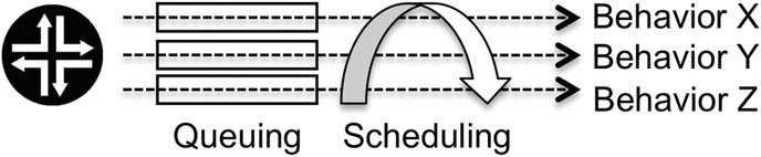
Figure 3.3 Each queue associated with the scheduling policy provides a specific behavior
As also discussed in Chapter 2, other tools can have an impact in terms of delay, jitter, and packet loss. However, the queuing and scheduling stage is special in the sense that it is where the traffic from different queues is combined into a single output.
So if, after taking into account the required behavior, traffic is aggregated into classes of service, and if each queue associated with the scheduling policy provides a specific behavior, then mapping each class of service to a specific queue is recommended. A 1 : 1 mapping between queues and classes of service aligns with the concept that traffic mapped to each class of service should receive a specific PHB.
Also, if each class of service is mapped to a unique queue, the inputs for the definition of the scheduler rules that define how it serves the queues should themselves be the class-of-service requirements.
When we previously discussed creation of the classes of service, we considered that all traffic classified into a specific class of service has the same behavior requirements. However, as we saw in Chapter 2, the application of the CIR/PIR model can differentiate among traffic inside one class of service. A 1 : 1 mapping between queues and classes of service can become challenging if some traffic in a queue is green (in contract) and other traffic is yellow (out of contract). The concern is how to protect resources for green traffic. Figure 3.4 illustrates this problem, showing a case in which both green and yellow traffic are mapped to the same queue and this queue is full.

Figure 3.4 Green and yellow traffic in the same queue
As shown in Figure 3.4, the queue is full with both green and yellow packets. When the next packet arrives at this queue, the queue is indifferent as to whether the packet is green or yellow, and the packet is dropped. Because yellow packets inside the queue are consuming queuing resources, any newly arrived green packets are discarded because the queue is full. This behavior is conceptually wrong, because as previously discussed, the network must protect green traffic before accepting yellow traffic.
There are two possible solutions for this problem. The first is to differentiate between green and yellow packets within the same queue. The second is to use different queues for green and yellow packets and then differentiate at the scheduler level.
Let us start by demonstrating how to differentiate between different types of traffic within the same queue. The behavior shown in Figure 3.4 is called tail drop. When the queue fill level is at 100%, the dropper block associated with the queue drops all newly arrived packets, regardless of whether they are green or yellow. To achieve differentiation between packets according to their color, the dropper needs to be more granular so that it can apply different drop probabilities based on the traffic color. As exemplified in Figure 3.5, the dropper block can implement a behavior such that once the queue fill level is at X% (or goes above that value), no more yellow packets are accepted in the queue, while green packets are dropped only when the queue is full (fill level of 100%).

Figure 3.5 Different dropper behaviors applied to green and yellow traffic
Comparing Figures 3.4 and 3.5, the striking difference is that, in Figure 3.5, once the queue fill level passes the percentage value X, all yellow packets are dropped and only green packets are queued. This mechanism defines a threshold so when the queuing resources are starting to be scarce, they are accessible only for green packets. This dropper behavior is commonly called Weighted Random Early Discard (WRED), and we provide details of this in Chapter 8.
The second possible solution is to place green and yellow traffic in separate queues and then differentiate using scheduling policy. This approach conforms with the concept of applying a different behavior to green and yellow traffic. However, it comes with its own set of challenges.
Let us consider the scenario illustrated in Figure 3.6, in which three sequential packets, numbered 1 through 3 and belonging to the same application, are queued. However, the metering and policing functionality marks the second packet, the white one, as yellow.

Figure 3.6 Using a different queue for yellow traffic
As per the scenario of Figure 3.6, there are three queues in which different types of traffic are mapped. Q1 is used for out-of-contract traffic belonging to this and other applications, so packet 2 is mixed with yellow packets belonging to the same class of service, represented in Figure 3.6 as inverted triangles. Q2 is used by green packets of another class of service. Finally, Q3 is used by packets 1 and 3 and also by green packets that belong to the same class of service.
So we have green and yellow packets placed in different queues, which ensures that the scenario illustrated in Figure 3.4, in which a queue full with green and yellow packets leads to tail dropping of any newly arrived green packet, is not possible. However, in solving one problem we are potentially creating another.
The fact that green and yellow traffic is placed into two different queues can lead to a scenario in which packets arrive at the destination out of sequence. For example, packet 3 can be transmitted before packet 2.
The scheduler operation is totally configurable. However, it is logical for it to favor Q2 and Q3, to which green traffic is mapped, more than Q1 which, returning to Figure 3.6, has the potential of delaying packet 2 long enough for it to arrive out of sequence at the destination, that is, after packet 3 has arrived. Packet reordering issues can be prevented only if traffic is mapped to the same queue, because, as explained in Chapter 2, packets cannot overtake each other within a queue.
The choice between the two solutions presented above is a question of analyzing the different drawbacks of each. Using WRED increases the probability of dropping yellow traffic, and using a different queue increases the probability of introducing packet reordering issues at the destination.
Adding to the above situation, the queuing resources—how many queues there are and their maximum length—are always finite numbers, so dedicating one queue to carry yellow traffic may pose a scaling problem as well. An interface can support a maximum number of queues, and the total sum of the queue lengths supported by an interface is also limited to a maximum value (we will call it X), as exemplified in Figure 3.7 for a scenario of four queues.

Figure 3.7 Maximum number of queues and maximum length
The strategy of “the more queues, the better” can have its drawbacks because, besides the existence of a maximum number of queues, the value X must be divided across all the queues that exist on the interface. Suppose a scenario of queues A and B, each one requiring 40% of the value X. By simple mathematics, the sum of the lengths of all other remaining queues is limited to 20% of X, which can be a problem if any other queue also requires a large length.
3.3 Inherent Delay Factors
When traffic crosses a network from source to destination, the total amount of delay inserted at each hop can be categorized in smaller factors that contribute to the overall delay value.
There are two groups of contributors to delay. The first group encompasses the QOS tools that insert delay due to their inherent operation, and the second group inserts delay as a result of the transmission of packets between routers. While the second group is not directly linked to the QOS realm, it still needs to be accounted for.
For the first group, and as discussed in Chapter 2, two QOS tools can insert delay: the shaper and the combination of queuing and scheduling.
Let us now move to the second group. The transmission of a packet between two adjacent routers is always subject to two types of delay: serialization and propagation.
The serialization delay is the time it takes at the egress interface to place a packet on the link toward the next router. An interface bandwidth is measured in bits per second, so if the packet length is X bits, the question becomes, how much time does it take to serialize it? The amount of time depends on the packet length and the interface bandwidth.
The propagation delay is the time the signal takes to propagate itself in the medium that connects two routers. For example, if two routers are connected with an optical fiber, the propagation delay is the time it takes the signal to travel from one end to the other inside the optical fiber. It is a constant value for each specific medium.
Let us give an example of how these values are combined with each other by using the scenario illustrated in Figure 3.8. In Figure 3.8, at the egress interface, the white packet is placed in a queue, where it waits to be removed from the queue by the scheduler. This wait is the first delay value to account for. Once the packet is removed by the scheduler, and assuming that no shaping is applied, the packet is serialized onto the wire, which is the second delay value that needs to be accounted for.

Figure 3.8 Delay incurred at each hop
Once the packet is on the wire, we must consider the propagation time, the time it takes the packet to travel from the egress interface on this router to the ingress interface on next router via the physical medium that connects both routers. This time is the third and last delay value to be accounted for.
We are ignoring a possible fourth value, namely, the processing delay, because we are assuming the forwarding and routing planes of the router are independent and that the forwarding plane does not introduce any delay into the packet processing.
The key difference between these two groups of contributors to delay factors is control. Focusing on the first group, the delay inherent in the shaping tool is applied only to packets that cross the shaper, where it is possible to select which classes of service are shaped. The presence of queuing and scheduling implies the introduction of delay, but how much delay is inserted into traffic belonging to each class of service can be controlled by dimensioning the queue lengths and by the scheduler policy. Hence, the QOS deployment offers control over when and how such factors come into play. However, in the second group of delay factors, such control does not exist. Independently of the class of service that the packets belong to, the serialization and propagation delays always exist, because such delay factors are inherent in the transmission of the packets from one router to another.
Serialization delay is dependent on the interface bandwidth and the specific packet length. For example, on an interface with a bandwidth of 64 kbps, the time it takes to serialize a 1500-byte packet is around 188 ms, while for a gigabit interface, the time to serialize the same packet is approximately 0.012 ms.
So for two consecutive packets with lengths of 64 and 1500 bytes, the serialization delay is different for each. However, whether this variation can be ignored depends on the interface bandwidth. For a large bandwidth interfaces, such as a gigabit interface, the difference is of the order of microseconds. However, for a low-speed interface such as one operating at 64 kbps, the difference is of the level of a few orders of magnitude.
Where to draw the boundary between a slow and a fast interface can be done in terms of defining when the serialization delay starts to be able to be ignored, a decision that can be made only by taking into account the maximum delay that is acceptable to introduce into the traffic transmission.
However, one fact that is not apparent at first glance is that a serialization delay that cannot be ignored needs to be accounted for in the transmission of all packets, not just for the large ones.
Let us illustrate this with the scenario shown in Figure 3.9. Here, there are two types of packets in a queue: black ones with a length of 1500 bytes and white ones with a length of 64 bytes. For ease of understanding, this scenario assumes that only one queue is being used.

Figure 3.9 One queue with 1500-byte and 64-byte packets
Looking at Figure 3.9, when packet 1 is removed from the queue, it is transmitted by the interface in an operation that takes around 188 ms, as explained above. The next packet to be removed is number 2, which has a serialization time of 8 ms. However, this packet is transmitted only by the interface once it has finished serializing packet 1, which takes 188 ms, so a high serialization delay impacts not only large packets but also small ones that are transmitted after the large ones.
There are two possible approaches to solve this problem. The first is to place large packets in separate queues and apply an aggressive scheduling scheme in which queues with large packets are served only when the other ones are empty. This approach has its drawbacks because it is possible that resource starvation will occur on the queues with large packets. Also, this approach can be effective only if all large packets can indeed be grouped into the same queue (or queues).
The second approach consists of breaking the large packets into smaller ones using a technique commonly named link fragmentation and interleaving (LFI).
The only way to reduce a packet serialization delay is to make the packets smaller. LFI fragments the packet into smaller pieces and transmits those fragments instead of transmitting the whole packet. The router at the other end of the link is then responsible for reassembling the packet fragments.
The total serialization time for transmitting the entire packet or for transmitting all its fragments sequentially is effectively the same, so fragmenting is only half of the solution. The other half is interleaving: the fragments are transmitted interleaved between the other small packets, as illustrated in Figure 3.10.

Figure 3.10 Link fragmentation and interleaving operation
In Figure 3.10, black packet 1 is fragmented into 64-byte chunks, and each fragment is interleaved between the other packets in the queue. The new packet that stands in front of packet 2 has a length of 64 bytes, so it takes 8 ms to serialize instead of the 188 ms required for the single 1500-byte packet.
The drawback is that the delay in transmitting the whole black packet increases, because between each of its fragments other packets are transmitted. Also, the interleaving technique is dependent on support from the next downstream router.
Interface bandwidth values have greatly increased in the last few years, reaching a point where even 10 gigabit is starting to be common, so a 1500-byte packet takes just 1 µs to be serialized. However, low-speed interfaces are still found in legacy networks and in certain customers’ network access points, coming mainly from the Frame Relay realm.
The propagation delay is always a constant value that depends on the physical medium. It is typically negligible for connections made using optical fiber or unshielded twisted pair (UTP) cables and usually comes into play only for connections established over satellite links.
The previous paragraphs described the inherent delay factors that can exist when transmitting packets between two routers. Let us now take broader view, looking at a source-to-destination traffic flow across a network. Obviously, the total delay for each packet depends on the amount of delay inserted at each hop. If several possible paths exist from source to destination, it is possible to choose which delay values will be accounted for.
Let us illustrate this using the network topology in Figure 3.11 where there are two possible paths between router one (R1) and two (R2), one is direct and there is a second one that crosses router three (R3). The delay value indicated at each interconnection represents the sum of propagation, serialization, and queuing and scheduling delays at those points.

Figure 3.11 Multiple possible paths with different delay values
As shown in Figure 3.11, if the path chosen is the first one, the total value of delay introduced is Delay1. But if the second is chosen, the total value of delay introduced is the sum of the values Delay2 and Delay3.
At a first glance, crossing more hops from source to destination can be seen as negative in terms of the value of delay inserted. However, this is not always the case because it can, for example, allow traffic to avoid a lower-bandwidth interface or a slow physical medium such as a satellite link. What ultimately matters is the total value of delay introduced, not the number of hops crossed, although a connection between the two values is likely to exist.
The propagation delay is constant for each specific medium. If we consider the packet length to be equal to either an average expected value or, if that is unknown, to the link maximum transmission unit (MTU), the serialization delay becomes constant for each interface speed, which allows us to simplify the network topology shown in Figure 3.11 into the one in Figure 3.12, in which the only variable is the queuing and scheduling delay (Q&S).

Figure 3.12 Queuing and scheduling delay as the only variable
In an IP or an MPLS network without traffic engineering, although routing is end to end, the forwarding decision regarding how to reach the next downstream router is made independently at each hop. The operator has the flexibility to change the routing metrics associated with the interfaces to reflect the more or less expected delay that traffic faces when crossing them. However, this decision is applied to all traffic without granularity, because all traffic follows the best routing path, except when there are equal-cost paths from the source to the destination.
In an MPLS network with traffic engineering (MPLS-TE), traffic can follow several predefined paths from the source to the destination, including different ones from the path selected by the routing protocol. This flexibility allows more granularity to decide which traffic crosses which hops or, put another way, which traffic is subject to which delay factors. Let us consider the example in Figure 3.13 of two established MPLS-TE LSPs, where LSP number 1 follows the best path as selected by the routing protocol and LSP number 2 takes a different path across the network.

Figure 3.13 Using MPLS-TE to control which traffic is subject to which delay
The relevance of this MPLS-TE characteristic in terms of QOS is that it allows traffic to be split into different LSPs that cross different hops from the source to the destination. So, as illustrated in Figure 3.13, black packets are mapped into LSP1 and are subject to the delay value of Q&S (1) plus constant (1), and white packets mapped into LSP2 are subject to a different end-to-end delay value.
3.4 Congestion Points
As previously discussed in Chapter 1, the problem created by the network convergence phenomena is that because different types of traffic with different requirements coexist in the same network infrastructure, allowing them to compete freely does not work. The first solution was to make the road wider, that is, to have so many resources available that there would never be any resource shortage. Exaggerating the road metaphor and considering a street with 10 houses and 10 different lanes, even if everybody leaves for work at the same time, there should never be a traffic jam. However, this approach was abandoned because it goes against the main business driver for networks convergence, that is, cost reduction.
Congestion points in the network exist when there is a resource shortage, and the importance of QOS within a network increases as the available network resources shrink.
An important point to be made yet again is that QOS does not make the road wider. For example, a gigabit interface with or without QOS has always the same bandwidth, 1 gigabit. A congestion point is created when the total amount of traffic targeted for a destination exceeds the available bandwidth to that destination, for example, when the total amount of traffic exceeds the physical interface bandwidth, as illustrated in Figure 3.14.

Figure 3.14 Congestion point because the traffic rate is higher than the physical interface bandwidth. P, physical interface bandwidth
Also, a congestion scenario can be artificially created, for example, when the bandwidth contracted by the customer is lower than the physical interface bandwidth, as illustrated in Figure 3.15.

Figure 3.15 Congestion point artificially created. C, contracted bandwidth; P, physical interface bandwidth
At a network congestion point, two QOS features are useful: delay and prioritization. Delay can be viewed as an alternative to dropping traffic, holding the traffic back until there are resources to transmit it. As we saw in Chapter 2, both the shaper and queuing tools are able to store traffic. Delay combined with prioritization is the role played by the combination of queuing and scheduling. That is, the aim is to store the traffic, to be able to select which type of traffic is more important, and to transmit that type first or more often. The side effect is that other traffic types have to wait to be transmitted until it is their turn.
But let us use a practical scenario for a congestion points, the hub-and-spoke topology. Figure 3.16 shows two spoke sites, named S1 and S2, which communicate with each other via the hub site. The interfaces’ bandwidth values between the network and the sites S1, S2, and the hub are called BW-S1, BW-S2, and BW-H, respectively.

Figure 3.16 Congestion point in a hub-and-spoke topology
Dimensioning of the BW-H value can be done in two different ways. The first approach is the “maximum resources” one: just make BW-H equal to the sum of BW-S1 and BW-S2. With this approach, even if the two spoke sites are transmitting at full rate to the hub, there is no shortage of bandwidth resources.
The second approach is to use a smaller value for BW-H, following the logic that situations when both spoke sites are transmitting at full rate to the hub will be transient. However, when those transient situations do happen, congestion will occur, so QOS tools will need to be set in motion to avoid packets being dropped. The business driver here is once again cost: requiring a lower bandwidth value is bound to have an impact in terms of cost reduction.
In the previous paragraph, we used the term “transient,” and this is an important point to bear in mind. The amount of traffic that can be stored inside any QOS tool is always limited, so a permanent congestion scenario unavoidably leads to the exhaustion of the QOS tool’s ability to store traffic, and packets will be dropped.
The previous example focuses on a congestion point on a customer-facing interface. Let us now turn to inside of the network itself. The existence of a congestion point inside the network is usually due to a failure scenario, because when a network core is in a steady state, it should not have any bandwidth shortage. This is not to say, however, that QOS tools are not applicable, because different types of traffic still require different treatment. For example, queuing and scheduling are likely to be present.
Let us use the example illustrated in Figure 3.17, in which, in the steady state, all links have a load of 75% of their maximum capability. However, a link failure between routers R1 and R2 creates a congestion point in the link named X, and that link has queuing and scheduling enabled. A congestion point is created on the egress interface on R1.

Figure 3.17 Congestion point due to a failure scenario
Traffic prioritization still works, and queues in which traffic is considered to be more important are still favored by the scheduler. However, the queuing part of the equation is not that simple. The amount of traffic that can be stored inside a particular queue is a function of its length, so the pertinent question is, should queues be dimensioned for the steady-state scenario or should they also take into account possible failure scenarios? Because we still have not yet presented all the pieces of the puzzle regarding queuing and scheduling, we will analyze this question in Chapter 8.
As a result of the situation illustrated in Figure 3.17, most operators these days use the rule, “if link usage reaches 50%, then upgrade.” This rule follows the logic that if a link fails, the “other” link has enough bandwidth to carry all the traffic, which is a solution to the problem illustrated in Figure 3.17. However, considering a network not with three but with hundreds of routers, implementing such logic becomes challenging. Here the discussion moves somewhat away from the QOS realm and enters the MPLS world of being able to have predictable primary and secondary paths between source and destination. This is another topic that we leave for Chapter 8 and for the case studies in Part Three.
3.5 Trust Borders
When traffic arrives at a router, in terms of QOS, the router can trust it or not. The term trust can be seen from two different perspectives. The first is whether the information present in the packets is valid input for the classifier deciding the class of service to which the packets belong. The concern is assuring that the classifier is not fooled by any misinformation present in the packets, which could lead to traffic being placed in an incorrect class of service.
The second perspective is whether an agreement has been established between both parties regarding the amount of resources that should be used at the interconnection point. The question here is whether the router can trust the other side to keep its part of the agreement or whether the router needs to enforce it.
If two routers belong to the same network, it is expected that the downstream router can trust the traffic it receives from its neighbor and also that the neighbor is complying with any agreement that has been established. However, this is not the case at the border between networks that belong to different entities.
A trust border is a point where traffic changes hands, moving from using the resources of one network to using those of another network. The term “different” should be seen from a control perspective, not from a topology perspective, because it is perfectly possible for the same entity to own two different networks and hence to be able to trust the information they receive from each other at the interconnection points.
An agreement regarding resources usage usually is in place at trust borders. However, the network that receives the traffic cannot just assume that the other side is keeping its part of the agreement; it needs to be sure of it. So two conditions need to be imposed: first, any traffic that should not be allowed in the network because it violates the agreement should get no farther, and, second, traffic needs to be trusted before being delivered to the next downstream router, effectively before entering the network trust zone.
Let us illustrate the points in the previous paragraphs with a practical example. Assume that the service contracted by a customer from the network is a total bandwidth of 10 Mbps (megabits per second) and that two classes of service have been hired, voice and Internet, where voice packets are identified by having the marking X. Bandwidth in the voice class is more expensive because of assurances of lower delay and jitter, so from the total aggregate rate of 10 Mbps hired, the customer has bought only 2 Mbps of voice traffic.
Let us assume that the customer is violating the agreement by sending 20 Mbps of traffic and all packets are marked X, a situation which, if left unchecked, can lead to the usage of network resources that are not part of the agreement (see Figure 3.18).

Figure 3.18 The border between trust zones
Before allowing traffic that is arriving from the customer to enter the network trust zone, the border router needs to make it conform to the agreement made by limiting it to 10 Mbps and by changing the markings of packets above the rate hired for voice traffic.
The change of the packets markings is necessary because, following the PHB concept, the next downstream router applies the classifier tool, and packets with the wrong marking inside the trust zone have the potential of fooling the classifier and jumping to a class of service to which they should not have access. Another possible option is for the border router to simply drop the packets that contain an incorrect marking.
An interesting scenario is the one of a layered network, for example, MPLS VPNs, in which traffic is received from the customer as Ethernet or IP and transits through the network encapsulated inside MPLS packets. Here, the information contained in the Ethernet or IP packets header is not relevant inside the network, because the routers inspect only the MPLS header. We explore such a scenario in the case studies in Part Three of this book.
3.6 Granularity Levels
Routers inside a network fall into two main groups: routers that are placed at the edge of the network, commonly named provider edge (PE), and core routers, commonly named provider (P). From a QOS perspective, the key differentiation factor between PE and P routers is not their position in the network topology but the types of interfaces they have. A PE router has two types of interfaces, customer and core facing, while P routers only have the second type.
A core-facing interface is where the connection between two network routers is made, and a customer-facing interface is where the service end points are located. A core- or customer-facing interface is not required to be a physical interface. It can also be a logical interface such as, for example, a specific VLAN in a physical Ethernet interface.
The division between interface types is interesting because of the granularity levels that need to be considered at each stage. Let us start by considering the example in Figure 3.19, which shows three customers, numbered 1 through 3, connected to the PE router, on two physical customer-facing interfaces (P1 and P2), and where traffic flows to or from the other network router via a core-facing interface.

Figure 3.19 Customer- and core-facing interfaces
Customer 1 uses service A and customer 2 uses service B, and both services are classified into COS1. Customer 3 uses service C, which is classified into COS2. The physical interface P1 has two logical interfaces, L1 and L2, on which the service end points for customers 1 and 2, respectively, are located. The interest in differentiating between types of interfaces is being able to define the required granularity levels.
All traffic present in the network should always be classified to ensure that there is never any doubt regarding the behavior that should be applied to it. As such, the lowest level of granularity that can exist is to simply identify traffic as belonging to one class of service, which encompasses all customer services and any other network traffic mapped to that class of service. A higher level of granularity would be to identify traffic as belonging to a certain class of service and also to a specific customer.
A core-facing interface has no service end points because it operates as a transit point, where traffic belonging to multiple classes of service flows through it. As such, the granularity level required is usually the lowest one. A core-facing interface does not need to know which particular customer the traffic belongs to. Returning to Figure 3.19, the core interface has no need to be concerned if the traffic mapped into COS1 that crosses it belongs to service A or B or to customer 1 or 2. All it should be aware of is the class of service to which the traffic belongs, because, in principle, traffic from two customers mapped to the same class of service should receive the same behavior from the network. However, the core interface always needs to be able to differentiate between the different classes of service, COS1 and COS2, to be able to apply different behaviors to each.
As for customer-facing interfaces, the granularity level required is usually the highest. In Figure 3.19, two service end points are located on physical interface 1, so just knowing the class of service is not enough. It is also necessary to know the specific customer to which the traffic belongs. An interesting scenario is that of customer 3, who possesses the only service end point located on physical interface 2. For this particular scenario of a single service end point on one physical interface, the interface itself identifies the customer so the granularity level required can be the lowest.
It is important to identify the necessary granularity levels at each interface because this has a direct bearing on how granular the QOS tools need to be. In Figure 3.19, in the core interface, traffic belonging to the class of service COS1 can all be queued together. However, on the customer-facing interface 1, queuing should be done on a per-customer basis, because the same interface has multiple service end points.
In a nutshell, core-facing interfaces typically should have the lowest granularity level (i.e., these interfaces should be aware only of class of service) and customer-facing interfaces should have the highest granularity level (i.e., these interfaces should be aware of both the customer and the class of service). However, exceptions can exist, as highlighted for customer 3.
When designing the network and deciding which tools to apply on each interface, the required granularity levels make a difference when selecting which QOS tools are necessary and how granular they need to be. These choices are typically closely tied with the hardware requirements for each type of interface.
3.7 Control Traffic
So far, we have focused the discussion on QOS on customer traffic that transits the network between service end points. But there is also another type of traffic present, the network’s own control traffic.
There are two major differences between control and customer traffic. The first is that control traffic results from the network operation and protocol signaling and provides the baseline for the connectivity between service end points on top of which customer traffic rides. In other words, control traffic is what keeps the network alive and breathing. The second difference is that the source of control traffic is internal. It is generated inside the network, while the customer traffic that transits the network between the service end points comes from outside the network.
As a traffic group, control traffic encompasses several and different types of traffic, for example, that for routing protocols and management sessions.
Let us provide a practical example illustrated in Figure 3.20. Here, customer traffic crosses the network, and router A issues a telnet packet destined to router B. Also because a routing protocol is running between the two routers, hello packets are present.

Figure 3.20 Control traffic in the network
The two routers have different perspectives regarding the control packets. Router A has no ingress interface for them, because they are locally generated control packets. As for router B, the control packets arrive on a core-facing interface together with any other traffic that is being transmitted between the two routers.
Starting by looking at router A, how it deals with locally generated control traffic is highly vendor specific. Each vendor has its implementation regarding the priorities assigned to the traffic, the QOS markings of such packets, and which egress queues are used.
For router B, the classifier has to account for the presence of control traffic so that it can be identified and differentiated from the customer traffic. This is just like what happens with any traffic that belongs to a specific class of service.
It is good practice to keep the network control traffic isolated in a separate class of service and not to mix it with any other types of traffic due to its importance and unique character. Even if the behavioral requirements of control traffic are similar to those for other types of traffic, this is the only situation in which the similarities should be ignored and a separate class of service should be reserved for control traffic.
3.8 Trust, Granularity, and Control Traffic
We have been discussing several of the challenges that exist in a QOS network, including the trust borders between a network and its neighbors, the different granularity levels to be considered, and the presence of control traffic. Now we bring these three elements together and present a generic high-level view of a traffic flow across two routers.
In Figure 3.21, a unidirectional traffic stream (for ease of understanding) flows from customer site number 1 to site number 2. Packets belonging to this stream are represented as white packets, and the service is supported by two routers, named R1 and R2.
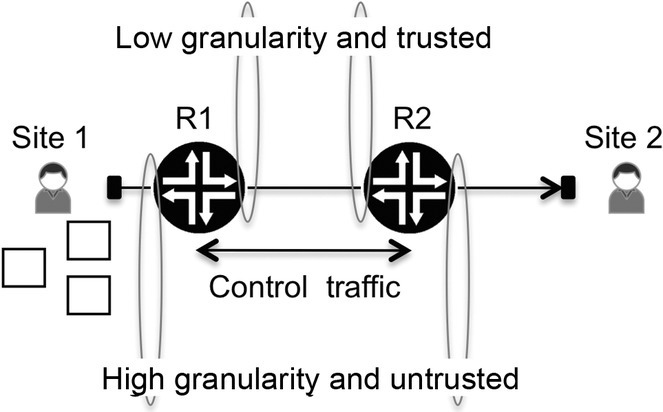
Figure 3.21 Traffic flow across two network routers
The first point encountered by the customer traffic flow is the service end point at the customer-facing interface on R1. This is the border between the customer and the service and, being a service end point, its granularity level is the highest so it should be customer aware.
Traffic originating from the customer is, in principle, considered untrustworthy, so the first step is to classify the customer traffic by assigning it to a class of service and to enforce any service agreements made with the customer, usually by applying the metering and policing functionalities or even more refined filtering based on other parameters that can go beyond the input rate of the traffic or its QOS markings.
Although traffic can be assigned to multiple classes of service, we assume in this example that it is all assigned to the same class of service.
The next interface is the core-facing interface that connects routers 1 and 2, which the customer traffic is crossing in the outbound direction. As with any core-facing interface, it should be class-of-service aware, not customer aware, in terms of granularity. The customer traffic is grouped with all other traffic that belongs to the same class of service and queued and scheduled together with it. Because it is a core-facing interface, in addition to customer traffic, network control traffic is also present, so the queuing and scheduling rules need to account for it. Optionally at this point, rewrite rules can be applied, if necessary, to signal to the next downstream router any desired packets differentiation or to correct any incorrect markings present in the packets received from the customer. This particular step is illustrated in Figure 3.22. Triangular packets represent control traffic packets that exist on any core-facing interface. White and black packets are mixed in the same queue because they belong to the same class of service, with white packets belonging to this particular customer and black packets representing any other traffic that belongs to the same class of service.

Figure 3.22 Queuing on a core-facing interface
Now moving to the core interface of router 2. The first step is classification; that is, inspecting the packets’ QOS markings and deciding the class of service to which they should be assigned. Being a core-facing interface, the classifier also needs to account for the presence of network control traffic. All the traffic received is considered to be trusted, because it was sent from another router inside the network, so usually there is no need for metering and policing or any other similar mechanisms.
The final point to consider is the customer-facing interface, where traffic exits via the service end point toward the customer. Being a service end point, it is typically customer and class-of-service aware in terms of granularity. At this point, besides the queuing and scheduling, other QOS tools such as shaping can be applied, depending on the service characteristics. This example can be seen as the typical scenario but, as always, exceptions can exist.
3.9 Conclusion
Throughout this chapter, we have focused on the challenges that the reader will find in the vast majority of QOS deployments. The definition of classes of service is a crucial first step, identifying how many different behaviors are required in the network and avoiding an approach of “the more, the better.”
Another key point that now starts to become visible is that a QOS deployment cannot be set up in isolation. Rather, it depends closely on other network parameters and processes. The network physical interfaces speeds and physical media used to interconnect the routers have inherent delay factors associated with them. Also, the network routing process may selectively allow different types of traffic to cross certain network hops, which translates into different traffic types being subject to different delay factors. So how the QOS deployment interacts with the existing network processes may limit or expand its potential results.
Further Reading
- Davie, B., Charny, A., Bennett, J.C.R., Benson, K., Le Boudec, J.Y., Courtney, W., Davari, S., Firoiu, V. and Stiliadis, D. (2002) RFC 3246, An Expedited Forwarding PHB (Per-Hop Behavior), March 2002. https://tools.ietf.org/html/rfc3246 (accessed August 19, 2015).