4 Microeconometric Analysis of Quality of Life and Living Standards

4.1 Types of consumer behaviour households and identification of key typological characteristics18

Following the pragmatic concept (see 1.2.4), while studying quality of life, we put at the forefront of the research the interaction of the needs (in the broadest sense of motivation Maslow’s “hierarchy of needs” [Маслов, 1999]) and the acual consumption. Accordingly, the problem of studying the differentiation of needs, manifested in different types of consumer behaviour of households, and the related problem of identifying the key typological characteristics can be attributed to the central problems of not only the theory and practice of consumer choice but the whole subject of the analysis of the quality of life of population.

Note that since this book is talking about an econometric approach, it is assumed that the proposed methodology should be implemented using specific socio-economic data. Available information sources of the issue discussed in this section are basically standard, official data from sampling of household budget surveys (SHBS), conducted quarterly by Rosstat of Russian Federation (RF). With respect to content, they cover, essentially, only the economic part of the above-mentioned Maslow’s “hierarchy of needs”. Therefore, the results presented in this section should be attributed to the analysis of economic well-being of the population, although the methodology itself with the necessary supportive information (which should include the results of additional questionnaire-type surveys of population) can be used to analyse the quality of life, understood in the most general sense.

4.1.1 Theoretical basis of research, source approval (hypotheses) and their formalization

(1°). First, our study is based on the so-called behavioural (statistical-genetic) approach, whereby the needs of the population, as a socio-psychological and economic category, should be studied, modelled and predicted by the analysis of the actual behaviour of consumers. The actual consumption and the real needs are formed in the household, the family – a social unit where specific interests, motives and orientations of people are refracted.

An alternative to the behavioural approach is a normative approach, the essence of which is reduced to an a priori (axiomatic) concept of needs, based on the postulates of physiology, psychology, health, architecture, etc. This approach underlines the calculations and design of the so-called statutory consumer budgets, claiming to define a set of vital needs of population. However, it conceals some controversy. Science can only formulate psychophysical requirements for the functioning of the human organism as a representative of a species. Thus, doctors, using the scientific method, can determine the number and the set of biologically active substances (proteins, fats, carbohydrates, salts, vitamins, etc.) required for the body and then normalize them for different population groups according to their gender, age, place of residence, the nature of work, employment, etc. Meanwhile, a person is a social phenomenon who functions as a member of society and has needs based not only on biological nature but is also connected with a whole complex of socio-economic factors, which are largely social. A human does not develop a need for specific nutrients (of which he may not even be aware) but for a specific set of foods. At the same time, the same combination of calories, proteins, fats and carbohydrates, vitamins, etc. could be realized by many different sets of foods varying by cost, nature, flavour and other qualities. Choosing the best, suitable, scientifically sound, rational, etc. from a plurality of possible combinations cannot be done using only scientific methods, from the standpoint of biological requirements of the organism. In this case, it is fundamentally important to take into account a wide variety of aspects of social conditions, and therefore, it is not surprising that the very task of identifying the needs transitions from the natural to the socio-economic sciences. The influence of environment and socio-economic factors has even greater impact on the formation of spiritual and intellectual needs. These needs are of a higher level and their role keeps increasing in modern society; they almost entirely depend on the development of society, culture, science, health, and social relations.

In addition, physiological norms underlying standard consumer budgets are defined autonomously and independently of each other for certain types of goods and services, whereas elements of the real structure of consumption are inseparable: the size and shape of the consumption of one type of goods and services affect the consumption of other goods. In other words, in reality, what we see are not separate needs but their complexes realized in stereotyped consumer behaviour.

Yet the truth is that we need a reasonable combination of behavioural and normative approaches. This, incidentally, concurs with the basic idea of Makarov [Макаров, 2010]. This basic idea “is to search and find in modern society the right balance between stiffness (in our case – the standard – S.A.) and flexibility (in our case – the freedom of choice of behaviour – S.A.), which provides stability of the system” (ibid. 11). Makarov states that “individual choice and collective choice are soft and hard components of the mechanism of distribution of wealth in human society” (42), and both of these elements, of course, must be present in such a mechanism. We are talking about standards in the broad sense (including social, energy-related, and environmental), far beyond food and other consumer products. Unfortunately, the very problem of the formation of standards is studied very poorly (Makarov calls it “a problem of the near future”, ibid. 45). We note only that the standards should be differentiated according to the considered types of consumer behaviour (or, in Makarov’s terms, “social clusters”). This, in particular, also follows from the well-known theory in the public sector of the economy, the “Tiebout hypothesis” [Tiebout, 1956].

(2°). Second, we proceed from the assumption that the society has an objectively conditioned socio-psychological and economic differentiation of population’s needs and the difference in consumption associated with it. The mechanism of this differentiation, functioning according to national particularities, socio-economic conditions, specifics of education and employment, and differences in culture and place in social production, although leading to ever greater individualization of consumption, acts in a way that generates a relatively small (compared to the millions of households considered) number of types of uniform consumer behaviour, covering the vast majority of consumption cells (households). Thus, we proceed from the objectively existing division of the totality of households into a number of similar (in terms of consumer behaviour) classes. Substantial (socioeconomic) explanation of this fact is based on the concept of group target structures of consumption and a related concept of targeted levels of consumption for each of the considered set of needs, first introduced by V. V. Soptsov [Митоян, 1990]. In particular, the existence of the target level of expenditures (consumption) of the analysed set of goods (services) is established using an empirical test of two requirements:

–	density of distribution of households according to expenditure per capita on this set of goods (services) must have a local maximum at a flow rate of the target level;
–	derivative of the regression function of income per capita according to the per capita expenditure on this set of goods (services) should abruptly increase when the flow value is equal to the target level.

The sufficiency of these conditions for the existence of the target level of expenditure per capita is determined by the fact that the first and second requirements may simultaneously be carried out only at the level of per capita expenditures, corresponding to the target level of consumption of this type of goods, but on other levels these conditions are not linked functionally or statistically. To understand this, we need to consider in more detail the content side of the above-mentioned requirements.

The first requirement, linking the target level of per capita expenditure on this group of goods with a maximum density of distribution of households according to per capita expenditures for the same group of products, has a fairly transparent meaningful interpretation. Indeed, the target level of consumption is determined by (and also defines) the existence of a centripetal force that has both a subjective and a socio-economic nature. This force causes the family not only to strive for a certain level of consumption but also to dwell on it for a certain period of time. This obvious mechanism results in an increased concentration of families in the neighbourhood of the point of per capita expenditure, corresponding to the target level of consumption of this type of goods. Having multiple target levels of household expenditure of families on the goods of the same commodity group (commodity complex) determines the appropriate number of local maxima of the density of distribution of households by per capita expenditures on this group of goods.

Meaningful interpretation of the second requirement of the existence of the target level of consumption is much less obvious. In this connection, we should consider this matter in more detail. Phenomenological research methodology of household consumption, which did not include the mechanism of formation of the consumer behaviour of households, has led to the concept of monotony and limited value of the function of expenditure/income dependency. This approach completely excludes the target aspect of consumption.

However, it is obvious that the family that has reached the target level of consumption of goods of a commodity group, for a period of time, does not increase its per capita expenditures for this group and channels increased per capita funds to expand its consumption of other commodity groups. This leads to the fact that in considering the regression dependency of per capita household expenditure on goods of a certain type (Y) from per capita income of the family (X), the regression line Υ on X, having reached the next target level cost Yl in the process of monotonic increase and then followed by further increase in per capita income, will still remain a time constant (Figure 4.1).

Levels of per capita expenditures Γ1 and Γ2 determine the upper limits of per capita expenditures, above which there are no families associated with the corresponding (Y1 and Y2) target levels of consumption of this type of goods.

Note the important fact that the function shown in Figure 4.1, i.e. the function of dependency of per capita expenditures on the goods of this complex on per capita income, is ambiguous. However, when constructing the regression of per capita expenditures of sample households on the selected goods over per capita income, this important feature does not manifest itself.

If levels of Y1 and Y2 correspond to the local maxima of the sample household distribution density on per capita expenditure on goods of the same group, then we have the sufficient condition that these levels (Y1 and Y2) are the target. Then the whole range of per capita expenditures of sample households for goods of the group is divided into three so-called consumer layers.

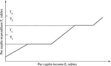
Figure 4.1. Regression of per capita expenditures on goods of one set to per capita family income as part of the study of consumption patterns

Yl – first target level of per capita expenditures;	Γ1 – the boundary of the first consumer layer;
Y2 – second target level of per capita expenditures;	Γ2 – the boundary of the first consumer layer;

The first target level corresponds to per capita expenditures of lower than Γ1 the second to per capita expenditures larger than Γ1 but lower than Γ2, and the third to expenditures larger than Γ2. Thus, any intersection (a combination in which each complex of goods is represented by one layer) of consumer layers of complexes of goods determines the consumer class.

(3°). Third, we rely on a provision conforming to which an actually folding pattern of consumption is the result of the desire of a multitude of households to optimize their satisfaction of needs and to make their consumption pattern most appropriate, and the optimality criterion (the concept of “the most appropriate” patterns of household consumption) is separate for each type (layer) of consumer behaviour.

Note that this position is essentially a basic concept also in the consumer choice theory, which uses the so-called objective preference functions (or consumption functions) as a tool to study the problem of consumption structure and forecast. However, the researchers operating in this area tended to overlook the need for a preliminary phase of research associated with the identification of the existing typological structure of consumer behaviour. In fact, the construction of preference functions (using budget data) is legitimate only when done separately for each type of consumer behaviour of households.

(4°). And finally, fourth, while evaluating the quality of life, we consider two aspects of causal attribution simultaneously: external circumstances and disposition of the analysed factor. At the same time, we remain on the positions of cognitive psychology just as proponents of the expansion of human giftedness concept. In our case, we are talking about the interaction of two multidimensional phenomena, one of which (disposition of the analysed factor) is the behaviour of the household in consumption area and the other (external circumstances) includes determinant factors that impact the formation of people’s needs.

Determinants are many and varied. On the one hand, they refer directly to the consumer, acting in the sphere of consumption. They are gender, age and family status, structure of population, social status and labour specifics of the people employed in social production and education level and preparedness to perform work of various qualifications. All of these factors to some extent determine social activity of the population in all spheres of life. On the other hand, determinants characterize the external conditions of consumer life and describe the consumption domain. They include climate; national-ethnic features; type of settlement (town, village, the capital, farm, etc.); conditions of distribution of material and spiritual values established in the community and reflected in the level and income inequality, in the use of public consumption funds, and the scope of the national wealth in the consumption sphere.

Of course, the above list of determinant factors is not intended to be exhaustive. In addition, we did not deliberately included factors describing the state of the productive forces, which indirectly affects the overall level of consumption. Ultimately, we will only be interested in the task of formalized description of dependencies that allow, using the values of the specific (if possible, concise) set of determinant factors, characterizing a household (HH), to predict to which type of consumer behaviour we can most likely refer to this HH. In addition, the identification of this set of determinant factors (which we shall henceforth call typological signs) is also included in this research.

* * *

Note that the statistical-genetic (behavioural) approach to identifying and explaining the structure of needs does not contradict the idea of the possibility of influence on the formation of the population’s needs of the society and, accordingly, does not rule out the regulatory role of the state in this process. On the contrary, the knowledge of the system of population preferences and its formal description allow to more clearly identify the boundaries and possibilities of exogenous influence on the actual development of the structure of demand.

From postulates (2°)–(4°), it is easy to conclude that the mathematical tool, the most suitable for model-formal description of the mechanism of differentiation of family consumption, identifying the main types of needs and consumer behaviour, definition of the main typological signs is multivariate statistical analysis, and particularly the sections such as cluster analysis, parameter estimation of mixtures of multivariate distributions, and reducing the dimensions of the tested feature space. Below is the language of some of the general concepts and basic assumptions of this research in terms of multivariate statistical analysis.

(A) The hypothesis of consumer unit: The actual consumption, as well as the real needs, is formed in the family (household) as the primary social unit in which interests, motivation and orientation of a person are refracted.

Based on this assumption, we come to a necessity to analyse consumer behaviour and the relevant determinants (factors of life) of the scope of families as a whole and each of them individually. In particular, let Oi, be a surveyed consumer unit (family) i; i = 1, 2, …, n, where n is the total number of analysed families. For brevity, we denote O = {Oi, i = 1,2,…, n} as the analysed scope of families.

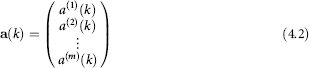
On examining living conditions (determinants) of the family 0„ in fact, we will » of the situation of family fix the values of a quantity (p) of indicators of the situation of family i. Among these p indicators (attributes) can be both quantitative (income, total number of family members, size of living area, age of family members, etc.) and qualitative or categorized (quality of housing, etc.) classification (profession of family members, the industry in which the head of the family works, the landlord, etc.). Thus, with each family 0„ we can associate a p-dimensional vector (or p-dimen-sional observation):

which is considered in the corresponding determinant space X (i.e. X∈X, i = 1,2, …,n).

Similarly, in the study of consumer behaviour (i.e. actually prevailing consumption patterns) of family 0„ we fix a certain number (m) of indicators of consumer behaviour, where denotes the specific (i.e. calculated on the average per family member) amount of ν type of goods (goods or services, including savings) consumed by the i family during the base period (year) and expressed in physical or monetary units.

Thus, each family Oi, is associated with Xi m-dimensional vector (m-dimensional observation):

which is considered in the corresponding space of consumer behaviour Υ (i.e.Y∈Y, i = 1,2, …,n).

To achieve the planned algorithmic scheme of the study, we need to make the spaces X and Y metric, or, in other words, to incorporate metrics into them (i.e. to determine the method of calculating the distance between any two elements in both space X and Y).

To arrive at the necessary initial mathematical concepts with which the given socio-economic categories and then setting their tasks are formalized, we need to clarify the wording of several abstracts.

(B) The hypothesis of the stratified nature of the behavioural space Y: It postulates the existence of a relatively small number of N types of consumer behaviour, such that the differences in consumption patterns of families of the same type are random (i.e. due to the influence of many random, uncontrollable or unaccountable factors) and insignificant compared to the differences in consumer behaviour of families from different types,

The geometric interpretation of hypothesis (B) means that there is a metric ρY(Oi, Oj) in the space Y, taking into account the nature of the relationship of the individual components of consumer behaviour yˆ and the proportion of their influence on the differentiation patterns of consumption that the whole given set of “multidimensional points” of O families in this space naturally decomposes into a relatively small number of point “clots”, or clusters which are “at a distance” (in the sense of the metric ρY), but do not break up into equally spaced parts.

(B°) A reinforced hypothesis about the stratified nature of space: It differs from hypothesis (B) by an additional assumption, according to which the random spread of multidimensional points, i.e. of families of consumer behaviour Yi(k), belonging to a (k-type) is subject to an m-dimensional normal law of probability distribution. In other words, if Y(k) is a random vector of consumer behaviour of a family, randomly extracted from a homogeneous set of families of k-type, then its probability density is given by a ratio:

In this ratio, vector

sets the average (and at the same time the most characteristic) structure of all possible consumer behaviours of the k-type households, and the matrix

determined by the so-called covariance of the components of consumer behaviour of k-type families, i.e.:

At the same time, the distribution of the random vector Y(k) is assumed to be non-degenerate.

Sample (empirical) analogues of theoretical values are and respectively:

where nk is the total number of households recorded in the k-type of consumer behaviour and is the value of the l component of consumer behaviour registered in the i-th k-family type.

(C) The hypothesis of optimality: This is the short term for the assumption according to which for every (k) type of consumer family behaviour we postulated the existence of its own optimality (or rationality) criterion, the mathematical expression of which is naturally presented in the form of the so-called preference function or target functions of consumption uk(Y). This function allows to numerically measure the degree of preference (rationality) of each fixed “consumer behaviour” Y, and the rules for calculating the numerical value of this degree of preference (i.e. the specific form of the consumption function) is the same only for the families belonging to the same type, and changes when we transition from one type to another.

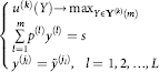
(D) Statistical manifestation of optimality hypothesis: It is a natural development of the optimality hypothesis (C). It postulates that the consumption structure Y, actually developed in a randomly selected family of k-type, is the result of objective laws (usually unconscious or only intuitively conscious by the family), equivalent to the evaluation and comparison of the different options for Y in terms of their degree of rationality. At the same time, a real measure of awareness of each individual family and the distorting effect of a set of random factors prevent it from reaching the exact optimal structure Yopt(k), but the objective trend of aspirations of a multitude of homogeneous (i.e. one type) families towards the optimization of their needs (under certain restrictions by income) is expressed in the fact that, as a result of the law of large numbers, the modal, i.e. the most commonly observed (in a broad class of cases it is the same as the statistical average) actual structure of consumption of households, k-type Ymod(k) is exactly optimal, i.e.

or is the same as

with restrictions

where p(1), p(2),…,p(m) are the retail price per unit of goods, respectively, y(1), y(2),…,y(m) and s(k) is the average value of the per capita average income of families (households) of the k-type of consumer behaviour (if specific quantities y(1),y(2),…,y(m) of goods consumed by the family are expressed in monetary units, then, obviously,p(1) =p(2) = … =p(m) = 1).

Equation (4.6) shows the limitations of resource type, while equation (4.6) shows the a priori restrictions on certain types of goods that are rationed or regulated. The relevance and obviousness of rationing and regulation of certain goods even in a market economy is clearly stated, for example, in [Makarov, 2010, sections 9.11–xs9.13]. However, they also mention (163) that “Mathematical economics has made a small contribution to the theory of rationing (see e.g. D.H. Howard Rationing, quantity constraints and consumption theory//Econometrica. 1977 Vol. 45. Ν 2.) There it is emphasized that the regulations distort the market equilibrium. Much more important is the question of how standards are generated by society.”

(E) The hypothesis of the existence of typological signs/determinants of the trust level (1–β): It is postulated that in the initial vector of factors of family life we can distinguish a sub-vector

and choose metric such as in the corresponding space X, and in this metric space, we can find non-overlapping domains for which the following statement is true: for any type of consumer behaviour there is the corre sponding range of values of typological signs , such that19

It is pertinent to note that the fulfilment of equation (4.7) allows to obtain an estimate of the accuracy of the method of determining the type of household consumption of the value of its typological sign. Namely, after the establishment of correspondences of type k↔t(k) between each of consumer type SY’ and the range of values of corresponding typological signs, we will determine the type of consumer behaviour for randomly selected family O* using the following rule: “from

it follows that

then from (4.7) we easily find that the number of incorrectly classified families cannot exceed ß.

4.1.2 General methodological logistics of the research

Solving the problem of the typology of consumer behaviour and identifying the main typological factors can now be represented as the following four phases of the general methodological logistics of the study, including the formulation of mathematical problems that must be solved at the same time.

Step 1. Collection and primary processing of raw data

As noted above, the source of information for solving the problem under discussion is the primary data (logs and diaries) from sampling of household budget surveys (SHBS) conducted quarterly by Rosstat RF and its regional agencies.

From the description of hypothesis (A) (see 4.1.1), we can see that the analysed objects (i.e. households – HH) act as multidimensional observations, or points, in two multidimensional feature space. On fixing as the coordinates of these points (HH) the values (or levels) of typological variables (i.e. the determinant factors), we see them in the space of the state , i.e. in the space of which the coordinates are the main indicators of family life. However, on fixing as the coordinates of the same points the indicator values of their consumer behaviour, we see them in the space of behaviour. Obviously, given the appropriate choice of the metric in spaces X and Y, the geometric proximity of the two points in space X will mean similarity of living conditions of the two respective families, and the geometric proximity of the points in space Y will show the similarity of their consumer behaviour.

Accordingly, at step 1, taking into account the specific characteristics of the original data {Xi,Yi}, i = 1, 2, …,n, it is necessary to solve the following two problems.

Problem 1. Selection of metric in space Y.

In other words, we are talking about the definition of a rule (algorithm), under which we have to calculate the “distance” between any two sets of consumer goods Yi and Yj. The success of this study largely depends on the successful solution of this problem. At the same time, we must not ignore the effect of essentially multivariate set of given behavioural traits YT = (y(1), y(2), …, y(m)). Let’s illustrate this idea with an example, which we artificially simplified (for clarity) by reducing the dimension of the given vector of consumer behaviour to two (i.e. let’s give YT = (y(1), y(2)) where y(1) and y(2) are the implied specific volumes of consumer goods categories “Food” and “Non-food”, respectively). The values (y(1) and y(2)) were recorded for each family in two different populations, and the families in “population I” differed significantly from the families in “population II” on a number of important factors of their life (income, geographic location, socio-demographic structure). Registration results are presented (on the conventional scale) in Figure 4.2, where the “crosses” are the geometric representation of population I and the “zeroes” of population II. Then, â1(I) and â1(II) are sample average expenditures of families I and II, respectively, for the category “Food”, and â2(I) and â2(II) are average expenditures of families I and II, respectively, for the item “Non-food products and other services”.

The statistical analysis showed that the component-wise difference of the means as well as the total component-wise difference of the means Δ1 + Δ2 is statistically significantly different from zero. In other words, if we focus on component differences without regard to their relationship, then it is not possible to establish a distinction in consumer behaviour of the two family populations. However, there is a difference and it is detected by using a metric that takes into account the nature of the relationships of the analysed components. In particular, based on the equity of the reinforced hypothesis of the stratified nature of the Y consumer behaviour space (hypothesis (B°)), make a natural assumption that the nature of the relationships between the components y(l)(k) and yq(k) (i.e. the covariance matrix Σ(k)) remains the same during the transition from one to another type of consumption, i.e.:

Then, the most natural metric, as we know (see, for example, [Айвазян, 2010], A3.3), is the distance of Mahalanobis type:

This is the metric we will use in space Y, especially because of its particular cases, corresponding to the diagonal covariance matrices of type

(which corresponds to mutually correlated componentsy1, y2,…,y(m) with the dispersions σ11, σ22, …, σmm) ¾d

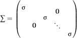
(which corresponds to mutually non-correlated components y№, y(2 …, y(mĩ with common variance σ) and, as is easily seen, it can be reduced to the weighted Euclidean metric

and the usual Euclidean metric

Problem 2. Reducing the dimensionality of space Y.

It refers to the transition from the m-dimensional vector Y for initial consumer behaviour characteristics to the vector Ỹ of the substantially smaller dimension m̃ (m̃≪m), the components of which, y(l), have to be formed as derived values from the initial characteristics y(1), y(2), …, y(m) (including ỹ(l) may repeat individual component of the vector Y), and at the same time be the most informative in terms of discovering the nature of differentiation of family consumer behaviour. The description of the methods for dimension reduction can be found, for example, in [Applied Statistics: Classification and dimension reduction, 1989]. In this problem, the formal methods of dimension reduction need to be combined with the methods of aggregation of the initial indicators, which are based on the content (socio-economic) analysis.

Step 2. Identification and modelling of the main types of consumer behaviour

The hypothesis that there are natural, objectively determined types of consumption, i.e. a number of family types with one class of families characterized by a relatively similar type of consumer behaviour, geometrically means disintegration of the set of points (families), studied in the behavioural space, into a corresponding number of bunches or clusters of points. Having identified these classes or clots using the methods of multivariate statistical analysis (method of cluster analysis, taxonomy), we obtain the basic types of consumer behaviour. And only after that we can constructively implement the method of constructing the objective preference functions, which develops and modifies the method proposed by V. A. Volkonsky [Волконский, 1973].

Accordingly, the realization of the objectives of phase 2 requires a solution to the following two problems.

Problem 3. Dividing a given population of households into a number (unknown to us) of classes so that the families belonging to the same class are characterized by a relatively similar consumer behaviour.

Mathematically, the problem is formulated as follows. There is a plurality of points {Yi}i =1,n in a multidimensional space Y and the metric ρY is defined in this space (using equation (4.8)). Starting from hypothesis (B) (or (B°)) of the stratified structure of population {Yi}i =1,n, we need to find a partition of this population SY into an unknown number JV of disjoint classes which (the partition), in a sense, would reproduce in the most accurate way the stratification structure. Obviously, such a formulation of the problem needs to be clarified; in particular, we need to explain in what way we are going to reproduce the desired stratified structure of the analysed population of families in the most accurate way.

Here are two versions of clarifying the statement of problem 3, depending on which hypothesis, (B) or (B°), will be used in this study.

If hypothesis (B) on the stratified nature of the behavioural space Y is true, problem 3 is solved by the method of cluster analysis, for example, using the procedure of “average JV” with an unknown number of classes Ν (see, e.g. [Айвазян, Мхитарян, 2001]). Ways to overcome the difficulties associated with the unknown number of classes and the search for stable (in some sense) types of partition are described in [Типология потребления, 1978, 59–68] (see also [Айвазян, 1996]).

If hypothesis (B°) on the stratified nature of the behavioural space Yis true, problem 3 is solved by using the procedures for estimating the parameters of normal distributions, followed by classification of observations Y1, Y2,…,Yn in accordance with the Bay es optimal decision rule. Indeed, hypothesis (B°) rules that the law of probability distribution of the whole given population O of multidimensional random points/families Y is a mixture of normal laws of probability distributions, each of which refers only to the families of one type of consumption. In other words, if f(Y) is probability distribution density of a multidimensional random variable describing consumption patterns randomly extracted from family O, then, in accordance with (B°)

where fk(Y) is the density of the m-dimensional (non-degenerate) normal law (see (4.1)), which (density) determines the laws of the random variation of the structure of k-type family consumption, and τk is the proportion (specific share) of k-type family consumer behaviour throughout the given family population O.

Obviously, in this case, the concept of a homogeneous class (type) of consumer behaviour (“strata”) is formalized with the concept of multivariate normal general population, and the task of the best partitioning of the given population 0 into disjoint classes is reduced to the best statistical estimation of parameters N, Tīfo a(k) and Σ (k)(k = 1,2, …,N) in equation (4.9). Indeed, knowing the parameters N, Tīfo a(k) and Σ (k) and taking into account (4.9), we have comprehensive information on the nature of each individual family consumer type and on their specific representation in the total population of families O. So in accordance with Bayes optimal classification rule, the i-th household (observation Yi) will be assigned to the class k0, for which

where the density of the m-dimensional normal distribution fk(Y) is defined by equation (4.1) (see the description of hypothesis (B°)).

Overcoming the challenges associated with an unknown number of classes JV and multi-variance of analysed distributions is described in Прикладная статистика: классификация и снижение размерности, 1989; Айвазян, 1997]..

Problem 4. Building the target functions of consumer preferences on the basis of family budget statistics.

The research methodology adopted for this study, as repeatedly noted above, is aimed mainly at (a) the identification of the nature of differentiation of consumer behaviour of population, (b) the development of analysis and prediction methods for this differentiation, and (c) the development of models that allow for partial management of consumer demand structure. If only the first two goals are undertaken, then to justify the use of the suggested methods in this book, it would be enough to rely on the assumptions in hypotheses (A), (B) (or (B°)), and (E). However, if we consider the desirability of moving on the path of socio-economic modelling, which allows to produce reasonable positive measures for the partial management of consumer demand, then one of the tools here is the use of retail prices, and, in particular, understanding the laws of their impact on demand. As it is well known [Слуцкий, 1963; Волконский, 1973, 1974], the most complete description of the patterns linking consumption (demand) volumes yl of various benefits to their retail prices pl and the income s can be obtained using target functions of consumer preferences u(k) (Y) (k= 1,2,…, N), which determine (up to a monotonic transformation) the numerical value of measure of optimality of each fixed set of benefits Y for families of k-type of consumer behaviour (see the formulation of hypothesis (C)). However, despite the presence of interesting and profound theoretical and methodological research on the analysis of the consumption functions [Frish, 1959; Слуцкий, 1963; Волконский, 1973, 1974], the attempts of their particular construction on the basis of statistical data have not been successful. Among the reasons for this situation, we can note the inadequacy and poor realism of key assumptions, which served as a basis of the given methods (see, e.g. [Frish, 1959], which postulates the “independence on preference”: the usefulness of one benefit does not depend on the amount of consumption of the other). The most promising in terms of application is the approach of V.A. Volkonsky, based on the so-called hypothesis of homogeneity [Volkonsky, 1973]. However, his attempts to statistically implement it on the total population of consumers, as expected, were unsuccessful for one simple reason: the homogeneity hypothesis suggests essentially the fulfilment of our hypotheses (A), (B), (C) and (D), but it is easily seen that these assumptions may be realistic only within a homogeneous consumer behaviour population of families. In the study [Volkonsky, 1973], this fact was not explicitly stated, and the remark, contained there, that the described “… models can in principle be applied also to specific classes of families somehow picked out from the main population” (p. 622) somehow leads away from the correct understanding of the valuable result formulated in the study: “cannot be applied …” (Emphasis added – S.A.), but must be applied only to certain classes of households, and not “somehow picked out from the main population” but picked out according to a certain criteria of homogeneity of their consumer behaviour. Thus, we arrive at the fact that within the framework of solving the general problem of identifying a typology of consumption and constructing consumer types as one of its aspects we can get the implementation of, what we think, is one of the most effective method of constructing the objective functions of consumer behavior based on data on family budgets.

We will briefly describe this method, relying largely on the work of [Volkonsky, 1973] and making some modifications arising from the comments just made.

We proceed from the assumption that hypotheses (A), (B°), (C) and (D) are correct. As initial statistics, we will consider family budgets of k-type of consumer behaviour (k= 1, 2, …, N), so that task 3 (the problem of partitioning of the whole analysed population of families O into classes on the basis of similarities in consumer behaviour of one class of families) is considered solved. Let’s assume Y(k) (m) is the general I couldn’t insert the real formula but Y should be capital and in bold, (k) is the power of Y and should be higher on the top of it and italic, (m) is fine as is..

Simultaneous execution of hypotheses (B°) and (D) guaranties, first of all, optimal statistical average of consumer behaviour of the families of each fixed (k) type, i.e. accuracy of the equation

and secondly, a normal character of the random scattering consumer behaviour vectors Y(k) not only in the totality of population of k family type (i.e. not only in the m-dimensional space Y) but in a narrower population of families Y(k)(m-l) selected from Y(k) (m), conforming to resource constraints (4.6). This means in particular that

where

is conditional expectation of a random vector f Y(k), calculated under condition (4.6), and Yопт.усл(k) the solution of the extreme problem such that

or, which is the same as

Note that the population Y(k) (m) is a subset of an m-dimensional space Y, while the whole population Y(k) (m-L-1) is a subset in a corresponding (m-L-1)-dimensional space.

In this situation, i.e. if hypotheses (A), (B°), (C) and (D) are accurate, the theoretical result proved in [Волконский, 1963] (see lemma on p. 632) can be used as the basis of a method of construction of quadratic approximation for the unknown function u(kY) on the statistics of family budgets. This result as applied to our study can be formulated as follows: if the random variation of the structure Y(k) of the consumer behaviour of families of k-type is adequately described by a non-degenerate m-dimensional normal law (see hypothesis (B°), formula (4.1)), and at the same time the structure Ymod(k), statistically more often observed in families of this type (in a symmetrical distribution, which includes normal, it is the same as the statistically average structure Yo(k)), is also optimal in the sense of (4.5), then in normal conditions and in the sense of (4.5–) the desired target function u(k)(Y) on the hyper-plane (i.e. while limited) can be replaced up to a monotonic transfortion by the density function fk(Y), and in particular

where the function

and the constants (for fixed income s) ck(s) and dk(s) are functions of s.

Hence, in particular, it follows directly that, on the whole, population Yˆ (m) (i.e. in the absence of restrictions on income) of the target function of the consumer behaviour of k-type households is a function of two variables ψk(Y) and s, i.e.:

while F(ψk, s) is a function, increasing for argument ψk.

To obtain a quadratic approximation of function uˆkY), let’s expand it into the Taylor series in the neighbourhood of the point a(k) up to a member of the second order inclusive, using expression (4.10), the rule for composite function differentiating, and the fact that

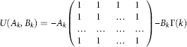
The result will be (up to a constant term and a constant positive factor):

In this equation, PT = (p(1), p(2), …,pm) is vector of retail prices20 and the constants A¾ and ¾ must be determined with some additional considerations.

To determine the unknown constants A¾ and ¾, we can use a combination of several approaches.

(a) Information on constants Ak and Bk contained in the postulate of “independences of preference” [Frish, 1959]. Mathematically, this postulate in relation to the benefits yl and y(q) is expressed by the following equation:

which should express the independence of utility of consumption of the benefit unit y(l) from the consumption of the benefit y(q) (but not the independence of the demand on benefit y(l) from the purchase volume of the benefit y(q) as the demand for all goods is interdependent through restrictions on income). The use of this postulate for all components (even with sufficient aggregation) of vector Y in order to build the consumption function u(k)(Y) [Frish, 1959] seems unjustified to us, because in this way, this assumption seems clearly unrealistic.

However, it is quite possible to select in a special way one or more individual pairs of the components

of vector Y (or pairs of suitably segregated initial components), such that for each of them the hypothesis of “independence of preferences” would be approximately accurate, i.e.

Using u(k)(Y) in the form (4.11), considering the matrix and assuming for definiteness that the components of vector Y are expressed in monetary units, we obtain from (4.12) the following system of equations:

By solving this system using the method of least squares, i.e. minimizing the sum

we can estimate only the equation τ = Ak/Bk. Its estimation is

(b) Information on constants A and B contained in the coefficient of elasticity of consumption by income. Under the elasticity el(k) l of the benefit y(l) by income (for k-type families), we understand a simple (not logarithmic) derivative of yl by s, that is

the actual value of which can be obtained, for example, from fairly statistically available demand functions (Engel curves) [Volkonsky, 1973].

Simple calculations associated with differentiating the optimized consumption function lead to the following system of equations for constants A and B:

where ε(k) = (e1(k), e2(k),…, em(k))T

is a matrix of size m×m, and lm = (1, 1, …, 1)T is an m-dimensional column vector of ones. Unfortunately, system (4.13) is difficult for finding the numerical solution and requires iterative procedures.

An example of the empirical study in which this method is implemented is presented in the work [Колосницын, Макарчук, 1982].

Step 3. Selection of the most informative determinant factors (typological variables) and stratification of households in the space of these variables

Obviously, it would be incorrect to rely on the fact that the range of possible values of each of the typological signs will not intersect for the families of different types of consumer behaviour. In other words, the values of each of the typological signs individually and their set of population are subject to some uncontrollable spread when analysing families within each type of consumption, i.e. they are characterized by some law of probability distribution. It is natural to consider the determinant factors or their sets as the most informative, the difference in the distribution of which is the greatest during the transition from one class of consumer behaviour to another. This idea is the basis of the selection method of the most informative typological signs. Finally, having already selected a small number of the most informative determinant factors, we can try again to partition the analysed family population into classes of clots but this time in the space of the selected typological signs. So, the result of this partitioning will depend not only essentially on the content of the group of the most informative typological signs but also on how we calculate the distance between two points/families in this space and, in particular, on the weight of the typological signs participating in this distance. Therefore, we will try to pick the weight so that the result of partitioning of families into classes in the space of the most informative determinant factors in a sense is the least different from the partition of the same points/ families that we obtained in the space of behaviour (step 2).

Step 3 of our logical plan, essentially, allows us to transition from the consumption typology to consumer typology and to find correspondence of these two structures. The result of this stage is the identification of the structure of the population by type of consumers determining the specific weight of each typological group. From the above, it follows that the content and the objectives of step 3 require solving the following two main problems.

Problem 5. The selection of the most informative (typological) variables in X space of determinant factors.

This problem is similar to task 2, which provided for the selection of the most informative factor in terms of identifying the differentiation of family consumer behaviour signs in the behaviour space Y. However, task 5 has two specific significant differences. First, p-dimensional signs analysed in space X are of mixed nature, i.e. we have quantitative, qualitative and classification signs included in the components of vector X. Ultimately, this difference in principle does not affect the overall statement of the problem, but creates only some additional complexity in the technical implementation of those elements of the logical solution of problem 2, which we may be needed to solve problem 5. The second difference is fundamental and, specifically, allows us to modify the general statement of the problem to make it possible to use a much more efficient method of selection of the most informative features than those used in task 2. It is a method based on the presence of the so-called training samples: in contrast to the conditions of problem 2, in problem 5 we are aware of the partitioning of these analysed objects (families) into homogeneous classes (types of use) before the analysis of the analysed system of signs X. Therefore, analysing the behaviour of various combinations of the components of X in different classes, it would be natural to name those most informative combination of these component behaviour changes dramatically during the transition from one class to another .

Let us illustrate this by describing a mathematical formulation of the problem. Let us have an original p-dimensional sign X = (x(1), x(2), …; x(p))Tof a mixed nature. In order to standardize the methods of algorithmic processing of all components simultaneously of vector X, let’s give to each component x(l) (l = 1, 2, … p) a finite set of its possible values (grades) x(l)(v)middle of the v-th grouping interval, into which the entire range of possible values of the random variable is a quantitative variable, thenx(l)(v) is the middle of the v–th grouping interval, into which the entire range of possible values of the random variable x(l) is divided; if xl is a sign of quality, then χ is the number of graduation, determining the level (degree of manifestation) of a given property or quality; and if j is a classification (nominal) sign, then x(l)(v)= v is the number of the class to which a particular object may be assigned. It is easy to calculate that the total number Μ of possible values of a multidimensional sign X is equal to the product mi·m1.--ţ. For a formalized description of differentiation of an occasional sign X, observed during the transition from one family class to another we need to introduce a quantitative measure for distinguishing between the classes in terms of this sign’s behaviour.

Content and experimental analysis of populations considered in the X space has led us in the long run to the most convenient and informative measure differentiation between the general household populations with numbers k1 and k2 to the so-called variation distance, given by the following equation:

where is the probability of occurrence of value Xi0 in j-th general population of families and the summing is performed for all m1.m2…mp possible values of the analysed characteristic X.

It is easy to check that the “distance” (4.14) is arranged in such a way that it is always non-negative and not greater than one, and Δ(k1 ,k2) = 0 if and only if Pk1(X) =Pk2(X), i.e. when the laws of probability of distribution of sign X in classes numbered k1 and k2 are identically the same.

Obviously, in our empirical analysis, we will have to use the sample analogues of values involved in (4.14), i.e.

where k(X) is the relative frequency of the occurrence (or fraction) among k-th population families of the kind of families, which have the value of the determinant factor that equals X, and the sum is carried out only by all values of X that have been registered at least once in corresponding populations.

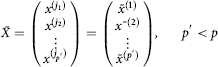
Then for each fixed dimension p′ = 1, 2, …, p−l and each possible set of components (the number of different sets of a given dimensions p′ equals the number of combinations of p elements of p′, i.e. we calculate the values and determine the most informative set of predetermined dimension η0 (θ) from the condition

or from the condition

In equations (4.15) and (4.15’)

and

where the “weight” of the pairs (k1, k2)of (k1, k2)classes are calculated by the formula

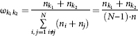
(here, as before, nk is the number of families classified as a result of solving problem 3 to the k consumption type).

We propose to select the dimension of the most informative sign among all the signs satisfying criterion (4.15) or (4.15’), using substantive socio-economic considerations. In addition, it is useful to trace the changes in the characteristic depending on p and to select for possible values of the dimension p′, primarily those for which there are “outstanding” in terms of value leaps in differences

Thus, by solving problem 5, we have found some p′ -dimensional signs the components of which are either selected from a number of initial determinant sign X or are some of its functions. This sign X can be considered as an experimental approach to some, not a priori known to us, typological signs, the existence of which is postulated by hypothesis (E). It will help us in the long run to determine (and to predict) the type of consumer behaviour of a family values using the values of its determinant factors.

Phase 3 is completed by the solution of the following problem.

Problem 6. Stratification of households in the space typological variables. The result of clustering of the analysed family population into disjoint classes in space depends not only on the composition of the components of vector of typological variables but also on how we calculate the distance ρ(Oi, Oj) between two points/families in this space.

We will introduce the distance between the objects specified by the multidimensional variables of mixed nature. We understand by the gradation of variables (l): for quantitative variables, it will be one of the grouping intervals, used to cluster the range of variation of the sign; for a qualitative sign, it will be one of the categories that define the quality of the analysed object; for a classification sign, it will denote one of the homogeneous groups (classes) into which the analysed population of objects is divided. Let m1 be the total number of possible gradations according to (l). Then each “observation”, as a result of the measurement of the variables (l) on the object Oi, will be conveniently represented by the binary vector where all components except one will equal zero. At the same time, the number of the single component v(l)(Oi) of vector is determined by the number of that gradation of the variables, in which the object Oi was included. We must set a measuring procedure to compute the measure of variation δ(l)(v1 ,v2) between –th and –th gradations of the variable When the grouping intervals and quality categories for quality and quantity variables are arranged in order, it is customary to use the following equation to denote this rate of variation:

where the value ci is a positive, “weight coefficient”, which reflects the relative measure of importance of the variables (l). In case of classification signs, we generally calculate this measure of variation by expert calculation. In the complete absence of meaningful considerations on the basis of which we could commensurate distances between different graduationsklasses in the case of classification components (l) we can propose, for example:

Then, the distance between the objects Oi and Oi, which are specified by multivariate observations Xi and Xi, respectively, is customary to set with the following equation:

where the “weights” cl, determining the relative value of separate components are the desired quantities and should be “matched” in the best, ı=ıso to speak, way, and the measure of variation of gradations δ(l)(v(l)(Oi), v(l)(Oj)), which include objects Oi and Oi on the variable (l) is calculated by means of (4.16), or by (4.16’)·

We need to find a weight vector for which the distance between the partitions SY and is the smallest, i.e.

In equation (4.18), the partition SY is the result of problem 3, i.e. classification structure of decomposition of the solution of problem 3, i.e. classification structure SY describes stratification of the analysed population of families O into the types of uniform consumer behaviour ,partition S-(C) is the result of the application of classification algorithms in space X of binary variables with metric defined by means of (4.16). A description of some classification algorithms of this type is given in Appendix 4.1.

Note. There are various ways to measure the distance between partitions (see, e.g. [Айвазян,Бежаева, Староверов, 1974; Миркин, 1976]). Here are two methods we used in the problem of typology of consumption. Let S(1) and (2) be two different partition classes of the same set of n objects.

Distance Kemeny-Snell dk-c (S(1),S(2)) is determined using the following formula:

where if objects Oi and Oj are in the same class of l-th partition, and sij (l)= 0 if the objects are in different classes of the l-th partition (l = 1, 2). It is easy to show that the values of the distance dk-c (S(1),S(2)) can vary from zero (when the partitions S(1)) and S(2)) coincide) to one (when one of the considered partitions n singleton classes, while the other unites all the objects into a single class).

Tanimoto distance dT(S(1) ,S(2)) (is basically equivalent to the distance Kemeny-Snell but in some cases is more convenient for computations) is defined by the following formula:

where n(l)(Oi) is the number of objects belonging to a class that contains an object Oi in the l-th partition and n(1.2)(Oi) is the number of objects and at the same time members of both of the aforementioned classes. It can be shown that the distance Tanimoto can vary from and it reaches its extreme values at the same partitions as the distance Kemeny-Snell.

An optimization problem (4.18) and the appropriate procedure for finding externum of function d(C) = d(SY, S(C)) of p′ is rather laborious. However, in this particular case, we can use the approaches that will significantly simplify this procedure and reduce the need of computer time to quite acceptable boundaries. We will describe one such approach.

Let’s consider identified vectors of most informative signs of the increasing dimension from 1 to p′ , found in the solution of problem 5, i.e.

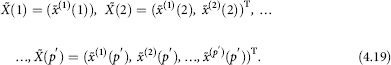
Let’s fix the components included in the “resulting” (i.e. finally selected) most informative p′ -dimensional sign and track how many times each of them occurs in a component of a sequence of vectors (4.19). Let μi be the total number of “occurrences” of the variable in the composition of the most informative sets (l), (2), …,(p′). Obviously l≤μi≤p′. Let us take as a zero approximation for the desired point of the externum value:

Let’s choose the step size δ (0,05,<δ<0,10) and on a part of the hyperplane let’s construct a “grid” with the nodes of the following form:

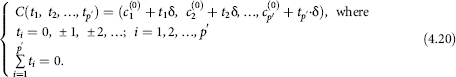
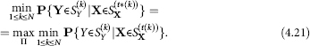
Further search for the minimum point (4.20) of the function d(C) is carried out by means of the directed enumeration of the values of the function at the nodes of the “grid” of the form (4.20). The search terminates at a point where the transition from any “neighbouring”21 grid point does not decrease the value of the analysed function.

We can see from the described solution of the problem of determining the best metric such as (4.17) in the space X that we also solve the problem of constructing the partition the least differing (in the sense of (4.18)) from the partition SY of the analysed population of families O into the types of consumption.

Step 4. Determination of the type of consumer behaviour of the household by the values of its typological variables

This step is devoted to, in essence, solving one problem, namely:

Problem 7. Achieving the best (in terms of the hypothesis (E)) equation of the partitions of the analysed population of households into classes in spacesX and Y.

We proceed from the understanding that we have already solved problems 1–6. Let’s define the substitution:

which shows a correspondence between the classes of the partition S(W̃) (see the description of hypothesis (E)) in such a way that it meets the following requirements:

In this relation, the empirical analogue (statistical evaluation) of the conditional probability is the percentage of those families among all families of class that entered into k-th type of consumer behaviour during the partitioning of the whole population of families O into classes in the space Y and the maximum on the right side is taken over all possible substitutions of . Thereafter, to simplify the record, let’s renumber the classes of the partition SX(C) SO that t * (k) = k. Knowing the substitution of * satisfying criterion (4.21), we automatically get the level of trust 1-β of typological determinant signs, see hypothesis (E)), which, considering renumbering of the classes, will be defined by the following equation:

Note. Formation of classes could be carried out without the search for metric ρ(c) and the partition S(C) in the space X, but using the usual Bayesian approach. Namely, the range of values Sk0 , getting into which “signals” the referring of the appropriate family to consumption type Sk0 is formed from all of these X values for which

As shown by the analysis and existing experience of experimental calculations, the results of the classification of households by type of consumption based on the values of their typological signs X using both these approaches are practically the same. However, the latter approach, i.e. the approach based on Bayesian criterion (4.22), is less convenient from the practical point of view.

Step 4 concludes the proposed methodological approach to the research of the typology of consumption.

4.1.3 An approach to forecasts of consumption macrostructure

Each of the separate steps 2–4 of the above methodology is dedicated to solving a problem, which, in itself, is of independent interest: whether it is about identifying the main types of consumer behaviour of households (step 2), the definition of the main factors that affect the selection of the household of a certain type of consumer behaviour (step 3), describing the functions of consumers’ preferences, according to which households of each type of consumer behaviour form their budget (step 2), or identifying the type of consumer behaviour of household values using characteristics of the household and environmental conditions such as its composition, average per capita income, place of residence, etc. (step 4). Realized as a complex, this methodology may serve as the basis for solving a number of urgent problems of the general theory and practice of consumption, demand and consumer choice.

As an example of one of these problems, we describe the general approach, based on this methodology, to a short-term (1–3 years) forecast of a macrostructure of consumption on the basis of the microeconomic data. The basis of this approach is an empirically verified statement, according to which the forecast of population structure in the space of determinant factors (which influence formation of human needs) is a much simpler task than the immediate forecast of behavioural characteristics of population. On this basis, the following logical micro-econometric research methodology is proposed.

1.	According to the initial data from SHBS for the current year, we implement steps 1–4 of the above methodology (task 4 of constructing objective functions of consumer preferences can be excluded in this case from step 2).
2.	With the help of well-known methods of forecasting socio-demographic structure of population, the employment structure and the structure of the geographic dispersal, we forecast (for 1–3 years) specific weights of the classes in the space of typological signs uncovered in step 3.
3.	Using the results of steps 2 and 4 on the values of typological variables, we determine types of consumer behaviour.
4.	Using the known average number of benefits, consumed by households of each type of consumer behaviour, and forecast values of specific weight of these types, we estimate the total number of each type of consumed benefit.