
Model assumption H4 states that the distribution of the population by per capita total expenditures x in the range of statistically unobservable values of these expenditures (i.e. where xi is the value of average total expenditures in the i-th statistically surveyed household, and n is the total number of statistically surveyed households) can be approximated by a three-parameter log-normal law with a parameter of the shift equal to ![]() and the parameter D(lnξ(k)) = σ2 independent of the number of stratum k and estimated by observations related to statistically surveyed strata of the population (see hypothesis H3).
and the parameter D(lnξ(k)) = σ2 independent of the number of stratum k and estimated by observations related to statistically surveyed strata of the population (see hypothesis H3).
Statement H4 is not a statistical hypothesis, since it cannot be directly statistically verified using a particular statistical criterion (the required statistics are not available). Therefore, statement H4 should be regarded an initial model assumption, the a priori validity of which can be justified only by suitable theoretical considerations and a posteriori by a comparison of the actual values of the main “output” characteristics with the corresponding values obtained on the basis of the proposed model. As theoretical considerations mentioned above, we can cite the following facts and evaluation of the specialists.
We can consider as one of the most significant consequences of the rapid collapse of the Soviet Union and its socio-economic system the formation of a narrow layer of “elite” from the highest ranks of party-bureaucratic and business elite, complemented by the most “advanced” representatives of organized crime, which, using specific methods of privatization, obtained the opportunity for overt and covert sales (on the international and domestic markets) of some appropriated items of national wealth. Various calculations of experts (see, e.g. [Suvorov, Ulianov, 1997]) show that “commodity intervention” on the markets of the national wealth in the amount of 0.2–0.3% of its physical volume (per year) is equivalent to an additional increase in the gross income of the population in the 10–20%. It is clear that the overwhelming share of the growth of gross income falls exactly on the stratum of the “elite”, which in view of the homogeneity of its social positions and the level of power can be classified as a specific socio-economic stratum. Therefore, the law of distribution of the population by expenditures, mentioned in assumption H4, refers to the population of this particular stratum.
Note that in normal circumstances we describe the distribution of the population by income (expenditures), with the income (expenditures) of this population exceeding a fixed level x0, using the Pareto law. However, it is justified only in cases where the probability density function of the total population decreases monotoni-cally for all x ≥ x0 (which, as a rule, takes place in a well-functioning economy). In case of the Russian situation in the 1990s, the above-described specifics of formation of the super-rich strata allows the existence of a local maximum of the density function to the right of point x0.
Using hypotheses H1 – H2 and assumptions H3 and H4 allows to build an informal (i.e. interpreted in terms of content) distribution model of the Russian population by per capita total expenditures and to design, based on this model, a methodology of statistical evaluation of poverty indicators and differentiation, based on the data from household budget surveys and some macroeconomic indicators of the balance of population income and expenditures.
Key variables used in the study and their information sources: Following the study [[Определение основных показателей, 1999], we define (in relation to the selected tact of time – a quarter) the cumulative monetary expenditure of HH as the sum of the following addends:
| – | ξ(1) quarterly consumer expenditures, as the sum of the costs of food, alcohol, non-food products for personal consumption of HH and for services of a personal nature; |
| – | ξ(2) expenditures of intermediate consumption (expenses of HH on personal subsidiary plots); |
| – | ξ(3) quarterly average gross of fixed capital of HH (purchase of land and real estate, precious metal products, costs of construction and renovation of housing); |
| – | ξ(4) quarterly sum of all paid taxes and other obligatory payments (including alimony, debt, club and society dues); |
| – | ξ(5) sum of balances of cash on hand and the growth of organized savings (including purchase of currency and securities and bank deposits); |
| – | ξ(6) cost estimation of quarterly consumption of products produced in personal subsidiary plots. |
Thus, the aggregate (total) per capita monthly expenditures ξ inadvertently extracted from the general population of households are
![]()
where mξ is the number of conventional consumer units in the sample households and the values ξ(l) (l = 1,2,..., 6) are defined above (additional division of the total sum of quarterly expenditures by 3 reduces the analysed random variable ξ to a more familiar factor for Russians, that is, monthly basis).
Note on the equivalence scales. The exact determination of the number mξ depends on the choice of the particular system of calculating equivalence scales. It is well known (see, e.g. [Equivalence Scales, Well-being, Inequality and Poverty]) that there are different approaches to the construction of equivalence scales. The Russian state statistical services, for example, calculate the value mξ based on the condition that children and family members of retirement age are estimated at, respectively, 0.9 and 0.6 consumer units. Equivalence scale OECD (Organization of Economic Cooperation and Development) is built on the principle of per capita income adjustment accounting for resource economy in the analysed income cell when jointly used. In accordance with this principle, the head of HH is given the weight of 1.0, other adults 0.7, and every child 0.5. Justification of the choice of a particular equivalence scale within the specificity of modern Russian society is a separate serious problem, which is outside of the scope of our study. In it, we determined that mξ simply equals the number of members of the analysed household.
The observed values ![]() of random variables, respectively,
of random variables, respectively, ![]() are the results of a statistical survey of the i-th household, obtained by standard SHBS Goskomstat and RLMS (fifth, sixth, seventh and eighth rounds). A macro-characteristic of total per capita expenditures of population on the region (μmacro) is derived from the quarterly “Balance of income and expenditures of population” of Goskomstat RF [Методологические положения по статистике, 1996]. The value μmacro has the same meaning and the same structure as the variable ξ. However, values μmacro and its components are calculated not with the sample statistics SHBS but with macro-regional trade statistics, tax services, banking information and securities market.
are the results of a statistical survey of the i-th household, obtained by standard SHBS Goskomstat and RLMS (fifth, sixth, seventh and eighth rounds). A macro-characteristic of total per capita expenditures of population on the region (μmacro) is derived from the quarterly “Balance of income and expenditures of population” of Goskomstat RF [Методологические положения по статистике, 1996]. The value μmacro has the same meaning and the same structure as the variable ξ. However, values μmacro and its components are calculated not with the sample statistics SHBS but with macro-regional trade statistics, tax services, banking information and securities market.
The relative frequency (share) ρ (x) of households with average and total expenditures x, evaded (or refused) from a statistical survey within the observation period, is assessed according to Goskomstat RF and RLMS (rounds 5–8). We also studied the parameters of the socio-demographic structure of families of the region (the regional average: the number of family members, share of children, the proportion of retirees, etc.).
Let's discuss in more detail RLMS data and SHBS, which were used as information source of our research.
1. Data RLMS, fifth, sixth, seventh and eighth rounds [Monitoring Economic Conditions in the Russian Federation, 1997]. These data on expenditures account for quite a broad range of categories, though the time ranges that include the expenditures of each category are different. For example, expenditures on food (about 60 positions) are calculated on a weekly window; fuel expenses, services (about 10), rent, club fees and insurance premiums, as well as savings and loans on a window of 30 days, and the cost of non-food products and durable goods (about 10 broad categories) on 3 months. RLMS maintains the records of food production at the personal subsidiary plots (for the previous year), together with the cost of its maintenance (facilities and equipment, fertilizers, seeds and purchase of seedlings, livestock and poultry, etc.). All these data are converted so that the resulting expenditures correspond to one calendar month. This “purified” data is published in the derivatives data files of RLMS.
Of course, the obtained results should be interpreted taking into account the quality of the source data. For example, the level of family welfare, as measured by the volume of consumption, should include the depreciation of consumer durables, real estate and vehicles; however, to our knowledge, this observation is only a theoretical possibility of the development of budget surveys, which is extremely difficult to implement.
2. The results of the sample budget survey by Goskomstat of households in three regions of the RF (second quarter of 1998), obtained in the course of the joint project of the working group CEMI and Goskomstat. According to the Goskomstat procedure [Определение основных показателей, 1999], the sample was formed on the principle of representative types of households on the basis of micro-census of 1994. Quarterly budget survey consists of a household filling a diary of expenditures for two weeks twice within the quarter and of an intermediate monthly survey. Based on the collected initial data on the expenditures, Goskomstat produces the following aggregate indicators, which will be used in the work: monetary expenditures (denras – the sum of actual expenses incurred by members of HH during the reference period –includes consumer expenditures and expenses not related to consumption); consumer spending (potras – part of the income for purchases of consumer goods and services); final consumption expenditures of households (konpot) and disposable HH resources (rasres – the sum of money, denres, and natural product, natdox, which were in possession of HH during the reference period, i.e. monetary expenditures, savings and natural products of HH deferred to the end of the accounting period). Budget surveys were also supplemented by a special questionnaire, for the research of the quality of life [Айвазян, Герасимов, 1998].
Description of the model and meaningful interpretation of its parameters. Let us use ξ (thousand rub.) to denote the average annual expenditure of randomly selected representative of the Russian population and ξj (thousand rub.) – the average per capita expenditure of the individual randomly selected from the population j-th homogeneous socio-economic stratum. Then, according to hypotheses H1 and H4, the distribution density of the random variable ξ is described by the model of a mixture of log-normal law such that
![]()
where ![]() are the parameters of the model, which could have the following meaningful interpretation:
are the parameters of the model, which could have the following meaningful interpretation:
k + 1 is the number of components of the mixture (each component is interpreted as a stratum of the population homogeneous by its socio-economic characteristics);
qj (j = 1,2, ..., k + 1) is the a priori probability of the appearance of observations, representing the j-th component of the mixture (the specific weight of the j-th homogeneous stratum in the entire population of the region);
x0 is a threshold value of per capita expenditures, separating statistically available range of change in expenditures (x ≤ x0) from statistically inaccessible range (x > x0);
aj = E(ln ξj) (j = 1, 2,..., k + 1) is the theoretical average values of logarithms of per capita expenditures (averaging is produced by the entire population of the j-th stratum);
![]() are the variances of the logarithms of average expenditures, calculated based on population of the j-th stratum.
are the variances of the logarithms of average expenditures, calculated based on population of the j-th stratum.
It is assumed that the entire population of (k + 1)-th (the richest) stratum has per capita expenditures that exceed a threshold value x0, and completely avoids sampling household budget surveys. The remaining households are available for statistical surveys, although they may evade (refuse) them with a probability ρ(x), where ρ(x) monotonically increases by per capita consumption function (see hypothesis H2).
Econometric analysis to identify model (4.39) implies, in particular, estimation of parameters Θ according to data from SHBS and “Balance of income and expenditure of population”.
Methodology of the econometric analysis of the model. Econometric analysis of the model implies, in particular (after the stage of its specifications, see below in this paragraph), statistical estimation of parameters. The peculiarity of this case lies in certain shortcomings of the necessary information support (i.e. data from SHBS), expressed in the evasion of the part of households slated for sampling survey from SHBS, including a complete absence in the sample of representatives of the “right tail” of the distribution ƒ(x |Θ) (in econometric literature, such problems are often called problems of selective sampling or the sample selection problem, see, e.g. [Вербик, 2008]). You can find more sources on the problems of information support of microeconometric analysis of the level and way of life of the population in Paragraph 4.4 below. Here, we touch on these issues only in connection with the problem of statistical estimation of parameters Θ of the function ƒ(x|Θ) defined by equation (4.39).
1. The probability p of evasion of a household from surveying as a function of some of its characteristics. In this section, we will focus on three characteristics as variables that determine the probability of evasion p
z(1) ln ξ is a logarithm (natural) of the total per capita expenditures of HH;
z(2) is a characteristic of the place of residence of HH (with gradations city, metropolitan areas, countryside and townships), which is represented in the model by three dummy variables z(2j) 1, 2, 3;
z(3) is a characteristic of the level of education of head of household (with gradations of below high school, high school, industrial and technical schools, technical and higher education), which is represented in the model by four dummy variables z(2.1) l = 1, 2, 3, 4.
Dependence of probability of evasion p from Z = (1, z(1), z(2.1), z(2.2), z(2.3), z(3.1), z(3.2), z(3.3), z(3.4),)T was analysed within logit-model of the following type:
![]()
where
![]()
and β = (β0, β1, β21, β22, β31,..., β34)T is the column vector of the desired (subject to statistical evaluation) model parameters (4.40).10 At the same time, characteristics z(1) and z(3) are introduced into the model in the form of dummy variables, so that after the econometric analysis of the model (4.40) the resulting function ρ (Ζ) gives us a whole set of models that describe the relationship between the probability of evasion from the surveys and the logarithm of total per capita expenditures z = z(1) at different combinations of gradations of variables z(2) and z(3). It will be convenient to define the elements of this set of functions with the help of
![]()
(obviously, the total number of such functions will equal 20).
In Appendix 4.2, you can observe the results of estimating the parameters β of function (4.40) according to RLMS data (rounds 5–8). Calculations confirmed a statistically significant monotonically increasing dependence of the probability ρ from z(1) with any combination of gradations of the associated variables z(2) and z(3) You can also see the results of econometric analysis of the simplification (paired) version of model (4.40), in which we analysed the dependence ρ only from z = z(1) In :
![]()
2. Calibration (weighting) of available observations. Analysis of the dependences (4.40) and (4.40″) may be interesting in itself. However, in our study, functions (4.40) and (4.40″) are used later to calibrate existing observations and distribution of the region (country) by total per capita expenditures, evaluated according to budget data: if the source data contains statistics for each (i-th) household surveyed in addition to the value of its total per capita expenditures and the “values” of associated variables ![]() then we can use for calibration function (4.40′) (where Ki and li are the numbers of gradations recorded, respectively, for the variables z(2) and z(3) in the i-th observation); if we have only the value of the total per capita expenditures, we have to be limited to the so-called rough calibration using function (4.40″). Taking this into account for future reference in order to simplify the notation, we shall denote functions (4.40′) and (4.40″) using ρ(z), in the case of calibration of logarithmized observed values of expenditures, and using ρ(x), if we have in mind calibration of the original observations (measured in thousand rub.).
then we can use for calibration function (4.40′) (where Ki and li are the numbers of gradations recorded, respectively, for the variables z(2) and z(3) in the i-th observation); if we have only the value of the total per capita expenditures, we have to be limited to the so-called rough calibration using function (4.40″). Taking this into account for future reference in order to simplify the notation, we shall denote functions (4.40′) and (4.40″) using ρ(z), in the case of calibration of logarithmized observed values of expenditures, and using ρ(x), if we have in mind calibration of the original observations (measured in thousand rub.).
Let ƒ (x) be a density function of distribution of the region's population by per capita expenditures. Then, η is the total number of statistically surveyed residents of the region and x* is a set value of per capita expenditures, and the number of observations v(x*) belonging to a small (of width Δ) neighbourhood of the point x* under the condition that no one evades the survey will look as follows:
![]()
Real (observed in the sample of volume n) number of observations ![]() calculated based on the known probabilities of evading survey ρ (x), will be
calculated based on the known probabilities of evading survey ρ (x), will be
![]()
From (4.41) and (4.42) it follows that
![]()
In particular, choosing as points x* the values of per capita expenditures xi (i = 1, 2,..., n), observed in the sample, and taking sufficiently small values Δ, we will have

And this means that if according to the available sample

we want to evaluate the true density function ƒ(x), then we have to transition to a weighed (calibrated) sample
![]()
where the weights ω¡ are determined by the formula
Note that the greater the weigh ωi is, the greater the probability of survey evading
p(xi), and ![]()
3. Estimation of the parameters of the statistically observable components of the mixture. At this stage, we are trying to solve the problem of estimating the parameters ![]() in a mixture of log-normal distributions of type
in a mixture of log-normal distributions of type
![]()
of sample (4.43). The problem is reduced to estimation of the same parameters in a mixture of normal distributions of the form
![]()
using the sampling
![]()
where zi = lnxi (i = 1, 2,..., n).
The results from solving this problem using the initial statistics of the eighth round of RLMS, as well as the data from household budget surveys of Komi Republic, Volgograd and Omsk regions (for the second quarter of 1998), are shown in the next section. The problem is solved by the method described in [Aivazian, 1996], using the results of [Dempster, Laird, Rubin, 1977] and [Rudzkis, Radavicius, 1995], with the software implemented in the packages “Classmaster” and STATA (for a brief description of the methods and algorithms, see Appendix 4.3).
4. Estimation of the unobserved component of the mixture and of the entire distribution as a whole. Let the specific weight of an unobserved ![]() component of the mixture be equal to
component of the mixture be equal to ![]() and the mean value of logarithms of per capita expenditures of this stratum be
and the mean value of logarithms of per capita expenditures of this stratum be ![]() Then, the overall average per capita expenditures μ for the entire population of the region calculated using model (4.39) accounting for the values obtained at the previous stage
Then, the overall average per capita expenditures μ for the entire population of the region calculated using model (4.39) accounting for the values obtained at the previous stage ![]() will be determined by the following formula:
will be determined by the following formula:

where
![]()
Taking into consideration the properties of the log-normal distribution, we obtained:
![]()
The value μ, defined by formula (4.44), depends on the unknown values ![]() and also on x0 and
and also on x0 and ![]() By construction, the value x0 shall be equal to the maximum observed value of per capita expenditures, i.e.
By construction, the value x0 shall be equal to the maximum observed value of per capita expenditures, i.e.
![]()
If hypothesis H′3 is true (see above), an overall estimation ![]() of the value σ2 is calculated using the following formula:
of the value σ2 is calculated using the following formula:
![]()
and the value ![]() shall be equal to
shall be equal to ![]()
Then, in the coordinate plane ![]() the level line is calculated from the condition:
the level line is calculated from the condition:
![]()
where ![]() is calculated using formula (4.44) with x0 = max1≤i≤n {Xi} “Balances of income and expenditures of population” for the analysed region and the corresponding tact of time.
is calculated using formula (4.44) with x0 = max1≤i≤n {Xi} “Balances of income and expenditures of population” for the analysed region and the corresponding tact of time.
The exact choice of ![]() on line (4.45) requires additional conditions or expert data. During the actual creation of the level line (4.45), it is useful to take into account the following considerations:
on line (4.45) requires additional conditions or expert data. During the actual creation of the level line (4.45), it is useful to take into account the following considerations:
| a) | from the general considerations it is evident that
(the symbol « means “considerably smaller”; in our case, we should state that qk+1 is approximately one order smaller than the value |
| b) | the level line (4.45) is created in the form of a table, in which the “input” is a grid of values
|
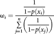
| c) | starting from (4.44), we can obtain the following upper bound value of the share of special weight q5 of the non-observed strata: |

Indicators of levels of poverty and social tension in the problem of targeted social support for low-income families. If we restrict the class of weighting functions w(x), involved in the expression of poverty indicators (4.35), by the functions of form (4.37), use the results of [Bourguignon, Fields, 1990] on the optimal allocation of a financial support to low-income families in this case and use the results of estimation of the density function ƒ(x) in terms of total per capita expenditures, then we can formulate the following optimal rule of targeted social assistance to the low-income families:
using the defined (“input”) parameters of the problem, that is, the total population N of the analysed region, the poverty line z0, the sum S allocated to target social support of the population, the density function ƒ(x) describing the distribution of the population in the region in terms of total per capita expenditures, and the value α > 1, narrowing down the Foster-Greer-Torbekka index used in the problem ![]() we will define the threshold value
we will define the threshold value ![]() from equation (4.38), i.e.:
from equation (4.38), i.e.:
![]()
every resident of the region with total per capita expenditures ![]() receives an allowance in the amount of
receives an allowance in the amount of ![]()
Clearly, a change in the appearance of the weighting functions w(x) can lead to the following modification in formulation of the optimal allocation rules of the targeted social assistance.
We calculated and analysed the proportion of the poor (i.e. indices of Foster– Greer–Torbekka ![]() when α = 0) and indicators of social tension (i.e. indices of Foster-Greer-Torbekka
when α = 0) and indicators of social tension (i.e. indices of Foster-Greer-Torbekka ![]() for α = 2) for each of the above-mentioned regions of Russia in three different ways:(1) through direct non-parametric estimations; (2) using estimates based on log-normal distribution model of population on per capita total expenditures and (3) using the estimates based on a model of log-normal distribution mixture. The results of these calculations and of the corresponding analysis are given in the following part.
for α = 2) for each of the above-mentioned regions of Russia in three different ways:(1) through direct non-parametric estimations; (2) using estimates based on log-normal distribution model of population on per capita total expenditures and (3) using the estimates based on a model of log-normal distribution mixture. The results of these calculations and of the corresponding analysis are given in the following part.
The results of the econometric analysis of the model. Formulated at the beginning of point 4.2.2, tasks 1, 2 and 3 and the methodology of this study described earlier led to the following general logistics of the econometric analysis:
| 1. | We conduct a non-parametric analysis of the distribution of population by total per capita expenditures on the basis of the data of Goskomstat of Russia for the second quarter of 1998 in the Komi Republic, Volgograd and Omsk regions (for each region separately), as well as according to the database of RLMS (eight round, data for November 1998) for Russia as a whole; on the “output” of this phase of research are histograms and basic numerical characteristics of the corresponding distributions (see Appendix 4.4). | ||||||||||
| 2. | On the basis of panel data from RLMS (five to eight rounds) on the evasion of households to participate in a survey11 within multiple and paired logit models, we evaluated the functions pkl (x) (see, eq. (4.40) and (4.40′)) and p (χ) (see formula (4.40″)), describing the dependence of the probability ρ of evasions of HH from surveying from on the value χ of its total per capita expenditures for various combinations of gradations of variables that determine the character of the country of residence of this HH, and the educational level of the head of HH (see Appendix 4.2). | ||||||||||
| 3. | In accordance with the above methodology we calibrate the source of statistical data: rough (i.e. using paired logit-model (4.40″)) for regional data and more refined (i.e. using multivariate logit model (4.40)) for nationwide data from RLMS, 8th round; with the goal of elimination of the shift in the assessment analysed l.d.p. caused by the effect of “survey evasion” within the statistical range of the observed values of average per capita expenditures HH (see introduction to Paragraph 4.2). | ||||||||||
| 4. | We repeat step 1, i.e. again we perform a non-parametric analysis of the analysed distributions, but this time based on calibrated data; the results are compared with the results of step 1. | ||||||||||
| 5. | In accordance with the above-described methodology, we estimate the parameters in models of mixture of distributions (three regional and nationwide) for calibrated data within the observed statistical range of the values of average total household expenditures (see Appendix 4.3). | ||||||||||
| 6. | In accordance with the methodology described above, we assessed the unobserved component mixture in each of the four analysed models (three regional and nationwide), with the goal of elimination of the shift in the estimation of analysed probability distribution caused by the effect of “truncation” outside of statistically observable range of values of total per capita expenditure of HH. | ||||||||||
| 7. | On the basis of distributions received in steps 4 and 6, we calculate and analyse indicators of poverty, and the differentiation of expenditures for the three regions under consideration (as of the second quarter of 1998) and for Russia as a whole (as of November 1998). We present below the results of this statistical analysis as in A4.1–A4.5 and Tables A4.2–A4.12 of Appendices 4.2 and 4.4, which show the following:
|
The analysis of the data in Tables 4.5 and 4.6 leads to the following conclusions:
| 1. | There is a substantial variation in the values of the analysed parameters between regions and (for each fixed region) between the methods of evaluation. In our view, the most accurate way to calculate the value of these characteristics is a non-parametric method of direct evaluation based on calibrated data (columns 8 and 9). And although it does not really change the ratings of the regions on these indicators, it provides significantly higher values of poverty indicators (for Komi Republic and Volgograd region it doubled!) than the official statistics. At the same time, the estimates derived from model of a mix yield in all cases the results significantly closer to direct non-parametric estimates than the official statistics, or a log-normal model. |
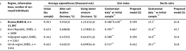
| 2. | Although the specific weight of the “non-observed” super-rich stratum included in the model is relatively small (in most cases it is measured in tenths and even hundredths of a percent), the impact of this stratum on the values of the key characteristics of differentiation and polarization of the population is significant. For example, the Gini index, according to official statistics, in November 1998, had the value of 0.380 for the country. For the straight non-parametric estimation of initial data RLMS (eighth round), it equaled 0.478. Having taken into account the latent stratum, its value increases to 0.599! The values of the Gini index by regions increase roughly by the same rate (with the exception of the Omsk region). The range of values of the decile ratio vacillates from 1.5 to 3 times. They are calculated using the shifted (unrepresentative) sample (column 8) and the model accounting for the latent stratum of the population (4.39) (column 9). |
Table 4.5. Indicators of poverty and social tension (Russia, November 1998)*
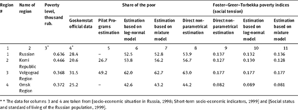
Table 4.6. The results of calibratio of distributions and the main indicators of differentiation by expenditures (Russia – as of November 1998, regions – as of the second quarter of 1998)
How do we explain the obtained differences and to what extent can we trust the results obtained on the basis of model (4.39)?
Table 4.5 shows the characteristics of poverty and social tension, the calculation of which is based on the “left tail” of the distribution of population expenditures. Therefore, as expected, the differences in the calculations made within an ordinary log-normal model and based on the mixture model (4.39) (compare columns 6 and 7, as well as 10 and 11) are quite small, though systematic (all values obtained from mixture model (4.39) are higher than the corresponding “log-normal” values by 1–2%). It is difficult to explain the spectacular differences between the “log-normal” characteristics and the official ones of the poverty level (compare columns 6 and 4): in fact, in accordance with Goskomstat methodology, such calculations would have to be made using exactly the log-normal distribution model! However, first, we used the RLMS data (eighth round), while the Goskomstat used the routine SHBS data of the fourth quarter of 1998, and second, the method for calculating the parameters of a log-normal approximation of distribution used by Goskomstat differs from the standard in mathematics and statistical practice.
Table 4.6 shows the characteristics of population differentiation by expenditures, the calculation of which is based simultaneously on two “tails” of the distribution – the left and right. And since one of the main salient features of mixture model (4.39) consists in a significant modification of the “right tail” of the distribution (by introducing and indirectly estimating the latent strata of the super-rich), the difference between the values of the characteristics of differentiation obtained by using model (4.39) (see columns 7 and 9) and the corresponding “Goskomstat” data (see columns 6 and 8) is, of course, quite impressive. Note that the results obtained by model (4.39) for the value of the Gini index and the funds coefficient may seem at first overly large. In support of this view, we can make the following observations. In model (4.39), the overwhelming proportion of the difference that exists between the μmacroŷ estimated by macro-statistics average value of per capita expenditures, and the value μ, obtained using SHHBS, can be explained by disregarding a latent “super-rich” stratum (compare numbers in parentheses in columns 4 and 5 in Table 4.6). If this share is too high, then the values of the Gini and funds coefficients, calculated by model (4.39), will turn out elevated.13 At the same time, in all the other approaches used to date, this difference is fully compensated by calibration of distribution within the statistically examined range of variation of the values of per capita income (expenses), which means a complete disregard for the existence of statistically unobservable population strata. Perhaps the truth lies somewhere between these two approaches? The answer to this question to some extent is contained in the following part.
The analysis of the stability of estimation of differentiation characteristics with respect to the systematic distortion of input data (the influence of the “misreporting” factor). Exaggerating the role of the non-observed strata in explaining the difference μmacro – μ in model (4.39) can occur, in particular, because of the systematic shift of sample survey data, due to the “misreporting” factor (see footnote 8). In other words, we are talking about deliberate lowering of their income and expenses by the respondents involved in the statistical sample surveys of HH.
In order to study the effects of the “misreporting” factor on the values of the Gini and funds coefficients derived from model (4.39) using data RLMS (eighth round) of Russia, we carried out the following calculations.
Let the distorting effect of the “misreporting” factor be measured by the value
![]()
where μcal (thousand rub.) is the average value of per capita household expenditures, estimated by sampling (within the observed range) and calibrated by the method described above in point 4.2.2 (in this case μcal = 0,932, see column 4 in Table 4.6) and μtruth (thousand rub.) – an unknown true average value of per capita expenditures represented in the sample of HH.
Obviously, our previous calculations (the results are presented in Tables 4.5 and 4.6, as well as in Tables A4.5-A4.8 of Appendix 4.3) give λ = 0, i.e. by assuming that μcal ≈ μtruth The total excess of expenditures μmacro over the calibrated expenditures μcal in the observable part of the range of the analysed sign is approximately 30% ((1.211 – 0.932)/0.932 = 0.299). The world practice of sample surveys of HH indicates that the mismatch of sampling and macroeconomic within several (usually less than 10) percent is a common phenomenon. In other words, it can be assumed that some of the difference μmacro _ μ still accounts for the available monitored range of the expenditure spectrum.
Table 4.7. Analysis of sensitivity of Gini index and funds coefficient towards the influence of the “misreporting” factor
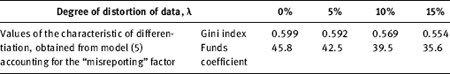
The results of calculations of the Gini index and funds coefficient, performed within model (4.39) for various values of, are given in Table 4.7.
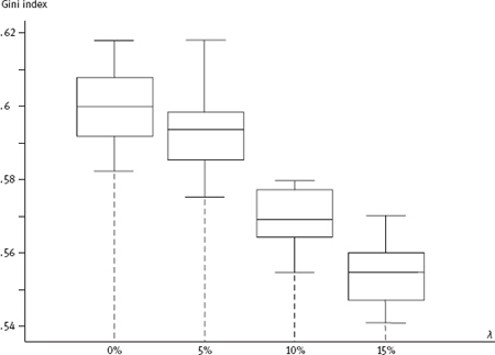
Calculations were made based on data generated using Monte Carlo simulation observation subordinate to distribution (4.39), in which the parameters σ2, aj, qj (J = 1, 2,..., k), ak+1 and qk+1 were estimated by the method described earlier in this paragraph and in Appendix 4.3 for sample RLMS data (eighth round)14 increased by λ%λ (each). For each value, we simulated 20 samples; the volume of each was 400.000. This volume of each sample was selected so that each latent stratum with the weight qk+1≤0,1% would have a sufficient number of representatives (about 100) in the sample. Presence of 20 samples for each value of λλ allowed to calculate the approximate scattered true values of estimated characteristics of differentiation, i.e. their interval estimates with a level of confidence no less than 0.95. Examples of such interval estimates are shown in Figure 4.5.
The results obtained show sufficient stability of the estimates based on model (4.39). Taking into account the comments made above and assuming quite realistic values of 10–15%, we can conclude that the values of the Gini and funds coefficients would most plausibly equal approximately to 0.55–0.57 and 36–39, respectively.
4.2.3 Modelling the mechanism for determining the distribution of families of average per capita savings
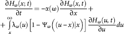
Let ω be a vector parameter that defines the type of family (its per capita income, number of people, socio-demographic structure), and ξω(t) be the average per capita value of savings, fixed in a randomly selected family ω and of “age” (the duration of the existence of the family in this type) t, hω(x;t) and Hω(x;t), respectively, the density function and the distribution function of the random variable ξω(t). We are interested in the limit (on t→∞) stationary distribution of family types ω(Hω(x) = Hω(x;∞)) and all families (h(x) = fhω(x) dP(ω))15 on per capita income variables and simultaneously in the dependence of basic value characteristics of the first family of distributions on the parameter ω.
As a model “entry”, let's introduce the following characteristics of consumption in the families of the type ω : α(ω) where α(ω) is the specific value (i.e. attributable to one family member per unit of time) of the “slow-moving” part of family income (in other words, this specific value of family funds, remaining after the necessary systematic expenditures on food, rent, etc.); and λω(x) is a characteristic of the intensity of spending of the slow-moving part of income in families with χ rubles of average per capita savings, i.e. during the time Δ t such expenditure takes place (purchase of durable goods – cars, country houses, expensive luxury items, where etc.). Then probability λω(x)·Δ t; Ψω(z|x) is a distribution function of the above-mentioned expenses occurring with the intensity λω(x).
The initial assumptions of the model are as follows:
| A) | The increasing (in time) process of monetary expenditures of the slow-moving part of the income is described by the jumping additive Markov process Zω(t|x) with the probability of a jump λω (x) and the distribution function of the jump value Ψω (z|x). |
| B) | Specifications α(ω), λω(x) and Ψω(z|x) satisfy the conditions that ensure the existence of a stationary distribution Hω(x), which is independent of the distribution Hω (x; 0) of the random variable ξω (0) .16 |
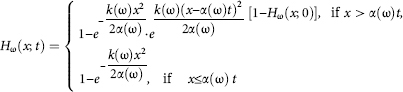
Affirmation. If the assumptions (A) and (B) are valid, then the distribution functions of the family per capita savings Hω(x; t) and Hω(x) are defined as the solutions of the following equations, respectively:
![]()
Corollary 1. If the function Ψis such that it allows the expansion
![]()
then
![]()
where cı and c2 are certain constants.
Corollary 2. If λω(x) = k(ω) x and Ψω(z|x) = z|x (i.e. the cost of one expenditure of the slow-moving part of the income is equally distributed within the interval of current savings x), then
and therefore
![]()
(known in technology as the Weibull distribution).
Corollary 3. Let us consider a simplified case in which the type of family is determined only by the value of its per capita income ω, and let us focus on the distribution of per capita value of savings of families whose income exceeds a certain predetermined level ω0. If the level ω0 is high enough (let's say not less than the average income, these very families present major interest to us from the point of view of savings), then the distribution of these households by per capita income η, as it is known, is well approximated by the Pareto law, i.e. by the distribution function of the form F(ω) = P(η < ω) = l-(ω0/ω)v. In this case, the transition from the distribution families of the given income group Hω(x), defined by (4.46), to the distribution of all families (with incomes in excess of ω0) by per capita savings yields (under additional assumptions α(ω) = α0.ω, λω(x) = λ(x) and φω(x) = ψ(x))
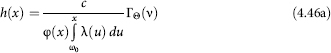
where ![]() is an incomplete gamma-function, and
is an incomplete gamma-function, and ![]()
The described model of the distribution of savings of the population can be taken as an object of econometric analysis. Special sample surveys of the population, “tuned” to this analysis, will allow statistical estimate of the “input” parameters of the model (α(ω), λω(x), Ψω(z)), to check the validity of the initial assumptions (A) and (B) and to conduct an experimental analysis of the results of its application.
4.3 Problems of information support of microeconometric analysis of the level and lifestyle of population
As we know, econometric analysis is based on the results of economic measurement. And if the accuracy and/or representation of these data are, for some reason, called into question, the results of the econometric analysis may also cause doubt. The main source of data of micro-econometric analysis in Russia is the national statistical office's quarterly sample surveys of household budgets (SHBS) carried out by state statistical services. They cover almost 50,000 households of the Russian Federation, distributed by regions (subjects of the RF) approximately proportionally to their population. Plans of sample surveys are drawn up in each region in accordance with the requirements of the regional representativeness of the sample and are implemented by regional state statistical services.17
In this section we will consider two tasks of analysis and correction of the results of sampling household budget surveys. The first task stems from the fact that in practice the results of SHHBS form a sample that, due to objective circumstances, always deviates from a representative (random) sample of the general population analysed in the region. We call this case the task of analysis and correction of sample survey data under the conditions of sampled selectivity (see explanation of this term below). The second task is generated by the aggregation defects that occur in the calculation of the average annual values of certain derivatives of these SHHBS characteristics of the respective quarterly averages. In other words, we are talking about the analysis and elimination of defects of temporal aggregation of the average values of the analysed indicators.
4.3.1 Data analysis and correction of selected sample surveys in the sample selection conditions
The main problems of the quality of information sources delivered by the results of SHHBS are related to the practical impossibility of implementation of a plan of sample survey, due to two factors:
| (i) | Among each stratum of population planned for survey, a certain percentage of household refuse surveying; |
| (ii) | Households with average monthly income exceeding a certain high enough threshold do not get in the sample, i.e. refuse surveying with the probability that equals one. |
These two facts lead to a shift based on sampling of results of econometric analysis in relation to the actual situation that characterizes the entirety of the analysed population. Accordingly, we are facing the task of a certain correction of SHBS data aimed at eliminating (or at least the maximum possible reduction) of this shift.
Both of these features of the SHBS data fall within the general problem known in econometrics and applied statistics as the sample selection problem (see, e.g. [Verbeek, 2008], 7.4 and 10.7). The essence of the problem is that certain objective conditions in the course of collecting the necessary sample data hinder the formation of a random (representative) sample, and this leads to the shift of statistical inferences based on this sample. In particular, the rule (necessary for the formation of a random sample) is violated, under which each of the elements of the analysed final general population of volume N falls into the sample with equal probability 1/N.
Obviously, some correction of such non-representative aiming at its approximation to the random one is only possible if there is some additional information, such as the parameters of the distribution of certain characteristics of the elements of the analysed general population, directly or indirectly associated with the analysed characteristics (in our case – with per capita incomes and household expenditures).
It should be noted that the fact (i) is more or less inherent in SHBS practice in other countries, while the circumstance (ii), meaning, in particular, the complete lack in the sample of the “right tail” of analysed the distribution of per capita expenditures (or income) can be attributed to the Russian specifics.
In the context of only one factor (i) we can obtain a satisfactory solution to the problem of correcting the existing survey results in order to eliminate (or at least minimize) the shift obtained on the basis of their using the methods of weighing the available survey data (see, e.g. [Deming, 1943; Kalton, Flores-Gervantes, 2003]). Among these methods, we select the most effective methods of family CALMAR (the methods for CALibration on MARgins, see [Zieschang, 1990; Deville, Särndal, 1992; Deville, Särndal, Sautory, 1993]). They are based on the implementation of the following ideas: the weights ω¡ for the i-th element of the sampling are selected in such a way that the weighted sample characteristics of the indicators, whose values are known for the general population (let's call these characteristics “control”), do not differ from the latter, subject to the least possible deviation (in some sense) of these weights from baseline.
However, with the simultaneous action of both factors (i) and (ii) the approach is incompetent, especially in solving problems of estimating various characteristics of differentiation of the distribution of population by average per capita income or expenditures, such as the funds or the Gini coefficients. In this case we propose a different approach.
You can see this approach below described in terms of a parametric formulation of the problem, i.e. in a situation where some general appearance of the analysed population distribution of per capita income or expenditure is postulated (in the given version a log-normal form of the distribution is postulated). Perhaps this approach could also be used for a semi-parametric case, i.e. to situations where only a general view of a “right tail” of the analysed distribution is postulated (which may be, for example, the Pareto distribution or a three-parameter, shifted log-normal distribution). Since we used the above-mentioned method of family CALMAR of weighing the available observations in the iterative procedure below, we will give a brief overview of this family of methods, adhering generally to the work [Deville, Särndal, Sautory, 1993].
Family of methods CALMAR of weighing the elements of a sample obtained under the conditions of a sample selection
Let us have observations
![]()
a random variable η, while sample (4.47) was formed in violation of the conditions to ensure its representativeness (randomness). This means that when we use the original weights di assigned to the observations yi we cannot guarantee the solvency of statistical inferences based on sample (4.47). So, generally speaking, the limit (at n→∞) ratios (of probability) will not be observed:
![]()
The general formulation of the problem can be presented as follows: it is necessary to fix the weights d= (d, d2,.... dn)τ so (i.e. it is required to find the new weights W = (wı, w2,.... wn)T) the sampled first moment of the analysed random variable η ![]() is as close as possible to (or exactly equal to) its theoretical first moment Eη while the new weights (W) would be in a sense, as closely as possible to the original (d).
is as close as possible to (or exactly equal to) its theoretical first moment Eη while the new weights (W) would be in a sense, as closely as possible to the original (d).
Additional information used to solve this problem by methods CALMAR is as follows: the formation of sample (4.47), along with the values of the analysed random variable η, we register the values ![]() i = 1, 2,..., n, of a range of supplementary (we'll call them “control”) random variables ξ = (ξ(1), ξ(2),...,ξ (k))T on each element of the analysed population; theoretical average values of these variables X0 = Eξ (Eξ(1), Eξ(2),......,Eξ(k))T are presented in macroeconomic data.
i = 1, 2,..., n, of a range of supplementary (we'll call them “control”) random variables ξ = (ξ(1), ξ(2),...,ξ (k))T on each element of the analysed population; theoretical average values of these variables X0 = Eξ (Eξ(1), Eξ(2),......,Eξ(k))T are presented in macroeconomic data.
In our case, average per capita income (expenditures) of the household is used as the analysed random variable η and as control variables we can use, for example, the same average per capita expenditures, proportion of children (under 15 years), retirees, etc. Obviously, the theoretical (general) averages of these control variables may be obtained from the macroeconomic statistics.
Mathematical formulation of the problem requires the introduction of the measure of distance ρ(d; W) between the initial (d) and sought (W) weights. It is determined by the following equation:
![]()
where the function G(z) must have the following properties:
G(z) is positive and strictly convex;
G(1) = G′(1)=0;
G″(l) = 1.
Then conditional optimization problem to minimize (in W) the distance ρ(d; W) provided that ![]() is reduced to the following problem:
is reduced to the following problem:
![]()
where λ = (λıλ2...λk)τ is the vector of Lagrange multipliers.
The solution of problem (4.49) is given in the following form:
![]()
where F(u) = g−1(u) (the inverse of the function g(z) = G′(z)), and the vector of Lagrange multipliers λ is determined by numerical methods from the system of equations:
![]()
(details of the corresponding computational procedure are described in Section 11 of the work [Deville, Särndal, Sautory, 1993]).
Note that the an inverse function of g(z) is provided by the properties of the function G(z), while F(0) = F′(0) = 1.
Here are the options for functions G(z) used in weighing observations by methods CALMAR:

where aminandamax are certain constants, such as Z∈ [amin, amax], while amin < 1 and amax > 1
![]()
Now we can proceed to the description of the proposed procedure for solving task 1 (see point 4.2.2), i.e. to the procedure of the analysis and correction of SHBS data to assess the distribution of the region's population by average per capita income (or expenditures).
Iterative procedure of simultaneous adjustment of weights W and estimation of the parameters of the analysed distribution
So, we have observations (yi, mi) (i = 1, 2,..., n0), where y¡ = lnsi, si is the value of average per capita income (expenditures) in the i-th surveyed household in the region, and mi is the number of members of the i-th household. At that time, the statistically available range of values s is limited on the top by s0 value (generally unknown). Assuming a log-normal distribution of the total population by per capita average expenditures s (i.e. in the full range of its possible values), we have the task of estimating the parameters a, σ2 and y0 = lns0 of the distribution density function of the logarithm of per capita income η = Ins among truncated on the right population of the region:
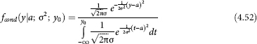
According to available observations from this “truncated” population:
![]()
where the multiplicity of valuer in the sample equals mi(i = 1, 2,..., n0).
Direct application of the maximum likelihood method to the data yi with weights ![]() does not provide consistent estimates for the unknown parameters due tdīĥe non-representativeness of sample (4.53). Therefore, a preliminary “reweighting” of the observations (4.53) using, for example, the procedure CALMAR18 and given macro-values (per capita) control variables z(3) β However, we know the values of control variables X0 for the entire general population, but to adjust the weights with the method CALMAR with a truncated distribution (4.52), we must use the corresponding values calculated only for a truncated (on top by expenditure) population of households. The share q(y0) of the “truncated” population is determined by the following equation:
does not provide consistent estimates for the unknown parameters due tdīĥe non-representativeness of sample (4.53). Therefore, a preliminary “reweighting” of the observations (4.53) using, for example, the procedure CALMAR18 and given macro-values (per capita) control variables z(3) β However, we know the values of control variables X0 for the entire general population, but to adjust the weights with the method CALMAR with a truncated distribution (4.52), we must use the corresponding values calculated only for a truncated (on top by expenditure) population of households. The share q(y0) of the “truncated” population is determined by the following equation:
![]()
i.e. it itself depends on the unknown parameters (a;σ2;y0). Therefore, we propose the following iterative procedure of simultaneous adjustment of weights W= (w1, w2,...,wn)T and of estimating the parameters (a;σ2;y0) of function (4.52).
The logarithmic likelihood function of estimations (4.53), subject to distribution (4.52), has the following form:
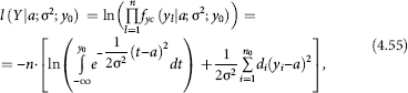
where ![]() and values yl form n0 series of identical elements yi in sample (4.53), the length of each series mi and the corresponding weight
and values yl form n0 series of identical elements yi in sample (4.53), the length of each series mi and the corresponding weight ![]()
The main idea of the proposed iterative procedure is as follows. Each (v-th) iteration consists of two parts. In the first part, using the above-described method CALMAR and set values of control variables, we estimate the weights W(v). In the second part of the iteration, using the weighted observations (4.53), we solve the problem of maximizing (for a; σ2 and y0) the likelihood function (4.55); using the obtained maximum likelihood estimations ![]() we estimate the share (4.54) population covered by the sample:
we estimate the share (4.54) population covered by the sample:
![]()
The procedure is iterative in nature, because before we start using it, we do not know what proportion of the population was not covered by the sample, and therefore do not know by how much the values of control variables X0 in the procedure CALMAR need to be truncated.
In the first part of the zero iteration in the CALMAR procedure in determining the weights W(0) = (w1(0), w2(0),..., wn(0))τ, we use not-truncated values of control variables X0· Since underestimated expenditures constructed from sample (4.53) can be explained by two factors (refusal to be surveyed by some proportion of the relatively wealthy part of households from the surveyed range of expenditures and the complete absence in the sample of households with average per capita expenditures in excess of the value smax), but we ignored the second factor at zero iteration, the weights wi(0) assigned in this iteration to relatively wealthy households of the statistically surveyed range of η variation will be somewhat elevated, and therefore, the share ![]() of the non-sampled rich population will be lowered. On the next (first) iteration in determining weights W(l) we will use as control variables Xo(l) already truncated values
of the non-sampled rich population will be lowered. On the next (first) iteration in determining weights W(l) we will use as control variables Xo(l) already truncated values ![]() Accordingly, the value of the weights wi(l) of relatively more affluent households of the surveyed range η will decrease. That means that as a result of the second part of the iteration the value of the share
Accordingly, the value of the weights wi(l) of relatively more affluent households of the surveyed range η will decrease. That means that as a result of the second part of the iteration the value of the share ![]() of non-sampled population will somewhat increase, etc. Empirically we established a very rapid convergence of this iteration process, i.e. while
of non-sampled population will somewhat increase, etc. Empirically we established a very rapid convergence of this iteration process, i.e. while ![]()
![]()
Note 1. In the work [Deville, Särndal, Sautory, 1993], the authors proposed several options to select the function of distance G(z) between the used (di) and sought weights (wi). They also describe computational algorithms and programs CALMAR to implement the method. However, as already mentioned, the problem is solved under the assumption that the observations are presented in the sample (households) of the total range of possible values of the analysed random variable. Therefore, in our formulation of the problem if we limit CALMAR data correction by weighing only, it will lead to inadequate (concentrated only in the surveyed, truncated on the top range of the analysed random variable) distribution law.
Note 2. In the work of [Sheviakov, Kiruta, 1999] they also considered the problem of estimating the problem of distribution of the population (households) in the region by per capita income (expenditures) based on unrepresentative data SHHBS. They essentially offer the option (2°) (see above) of weighing method CALMAR, but without the reference to the primary source. In that study the authors also ignore the complete absence of observations in the “right tail” of the analysed distribution.
Note 3. When implementing the second part of the proposed iterative procedure, it is useful to consider the following. On iteration zero when calculating the maximum likelihood estimates of parameters y0, a and σ2 you can use as zero approximation the following values:
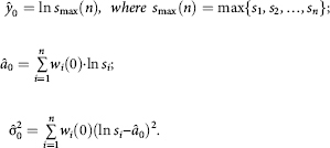
Then maximization (on y0, a and σ2) of log-likelihood function (4.55) is reduced to the minimization of the expression
![]()
in the vicinity of the point ![]() which may be accomplished, for example, with the method of grids.
which may be accomplished, for example, with the method of grids.
On any other (v + l)-th iteration we can use the same scheme with the replacement of variables ![]() by the values
by the values ![]() respectively.
respectively.
4.3.2 Analysis and elimination of defects in time aggregation average values
In this task, we are talking about a common practice in the statistical analysis of the aggregation defects that occur in the calculation of the average annual values of certain derivatives of SHHBS characteristics of the respective quarterly or monthly averages (see, e.g. [Scott et al., 2000]).19 For example, in accordance with the currently accepted methodology, the assessment q̄(x0) of the annual characteristic of the share of the poor q(x0) (i.e. the people whose per capita monthly income is below the “poverty line” x0) is defined as the simple average of the four values of the corresponding quarterly characteristics qi(x0) (i = 1. 2, 3, 4), i.e.:
![]()
We will show that with this method of calculation of the annual characteristics of poverty, we will always have a positive shift (assuming that the true share of the poor q(x0) < 0.5), i.e.:
![]()
where Δ(q(x0)) is a positive (at q(x0) < 0.5) systematic error, depending on the annual value of the true proportion of the poor q(x0), which in turn is determined by the parameters of distribution of the permanent component of per capita income.
Mathematical formulation of the problem and its solution
In accordance with the “permanent income hypothesis” of M. Friedman [Фридман, 1957], we assume that the average per capita monthly income ξi, characterizing a randomly taken individual in the i-th quarter of the year, is made up of the permanent (annual) component and a variable (quarterly) component δ¡, i.e.:
ξi, = ξ + δ¡ i = 1,...,4,
where quarterly components δ¡, being (as also is ξ) random variables, are independent of ξ and of each other and have mean values Eδ¡ equal to zero, and a constant (at i) dispersion σ2.
Let's introduce the density function (ƒ) and the corresponding distribution functions (F) for the law of probability distribution of the random variable ξ
(ƒξ(x) and Fξ(x)) and for the random variables δ¡ (fi(y) and Fi(y)). Then, using the known formulas, we can calculate the following probabilities:
So pı(xo) is the share (relative to the total population) of poor population at an annual rate, wrongly attributed, according to the results of the i-th quarterly survey, to the non-poor.
Similarly, ρ2(xo) is the share (relative to the total population of non-poor population at an annual rate, wrongly attributed, according to the results of the i-th quarterly survey, to the poor).
From the construction follows the formula linking the proportion of the poor in the annual (q(x0))and quarterly (q̄(xo)) basis:
![]()
Using the symmetry (relative to zero) l.d.p. of random variables δ¡ (i.e. Fi(y) = 1-Fi(–y)), and the fact that
![]()
where Z0 is the greater of the roots of the equation ƒ (z) = ƒ(x0), it can be shown that the value of the differenceρ2(xo)–p1(xo) is always positive.
Setting (or estimating) distributions of the random variables ξ and δ¡ (note that all δ¡, i = 1, 2, 3, 4 are identically distributed and mutually independent!), we can estimate the exact value of the shift in the assessment q(x0) of quarterly data. From the same distribution δ¡, in particular, follows that in this model the quarterly share of poor q¡(x0) remained virtually unchanged during the year (including deflated poverty lines and income).
Numerical example
Let the “poverty line” xo be set by the value xo = 3.5, and let (for ease of calculation) the random variables ξ and δ¡ be categorical variables with a finite number of values, and having the following symmetric l.d.p. (see Tables 4.8 and 4.9).
Table 4.8. The law of probability distribution of random variable
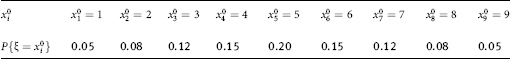
Table 4.9. The law of probability distribution of random variables δ¡
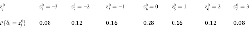
True annual characteristic q(x0) of the share of the poor is calculated directly from the set law of probability distribution in Table 4.8 of a random variable ξ:
![]()
Using the mutual dependence of the random variables and δ (and therefore, P{ξ = i, δ = j} = P{ξ = i}.P{δ = j}) and the laws of probability distribution of these random variables set in Tables 4.8 and 4.9, we will calculate p1 (x) and p2:
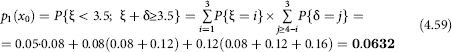
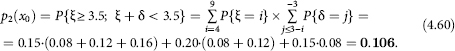
Placing the obtained values (4.58)–(4.59)–(4.60) in ratio (4.57), we see that the average quarterly estimate of the annual poverty level is about 4% higher than its true value.
Note 1. Having assessed using the available statistics dispersion σ2 of the quarterly variations in income around its permanent level, and setting, for example, a (0, σ2)-normal general appearance of a random variable δ¡ and a log-normal distribution value of permanent (annual) income, it is possible, using the scheme described above, to estimate the actual value of the shift.
Note 2. Using the same scheme, we can carry out the research of the problem of aggregation of monthly and quarterly data in the task of estimating the number of other characteristics of the analysed distribution, such as the dispersion and some indicators of differentiation (see, for example, performing similar tasks as well as some other approaches to their solution in [Scott, Strode, 2000]).
4.4 Conclusions
| 1. | The proposed concept of analysis of the problem of typology of household consumer behaviour is based on the hypothesis of the existence of the so-called targeted group consumption patterns and on the associated concept of targeted levels of consumption. This explains the fact that the mechanism of the objectively existing differentiation of needs of the population, operating according to national circumstances, socio-economic conditions, specifics of growing up and labour capacity, differences in culture level and place in the society lead (despite all the greater individualization of consumption) to a relatively small (compared with the total number of households) number of types of uniform consumer behaviour, covering the vast majority of households. | ||||||
| 2. | The behavioural approach to the identification and description of the existing types of consumer behaviour is an alternative to normative and is based on the empirical analysis on the actual behaviour of consumers. Mathematical tools used to implement this approach (including not only identification and description of the main types of consumer behaviour but also identification of those descriptive characteristics of the household, the so-called determinant factors, that mainly condition its assignment to a particular type of consumer behaviour) includes advanced methods of cluster and discriminant analysis. The specific implementation of the behavioural approach to Russian data in 1996 allowed to identify and analyse eight types of consumer behaviour, covering more than 85% of considered households (see Table 4.1) by the main determinant factor, the average per capita family income (see Table 4.2). | ||||||
| 3. | In the overall socio-economic system, which determines the nature of distributive relations in society, in accordance with objectively acting economic laws in the society (which in turn are caused by the main goals of the society, the adopted a system of values, etc.), we have a number of operating interrelated local mechanisms of individual socio-economic systems, such as (see Figure 4.3) blocks of distribution of workers according to their wages and entrepreneurs – according to business income; block of the structure of social consumption funds (the share of public funds allocated for health care and culture, for state family assistance, transport and etc.); blocks of retirees distribution by pension size, scholarship recipients – by scholarship size, families – by supplementary (“other”, i.e. not part of the wages, pensions or scholarships) cash benefits; block of distribution of families by the size of average per capita income; block of distribution of families by the size of average per capita savings; the block of socio-demographic and quantitative family structures and the block of structure of demand by population for various types of goods and services and their consumption. | ||||||
| 4. | The bio-anthropological model of the distribution of employees by salary size, considered in 4.2.1, in contrast to the common formal adaptations of existing experimental data into one of the theoretical models, describes the genesis, i.e. the very mechanism of formation of the analysed distribution, implemented within the initial assumptions operating under objective economic laws (their formalization is presented by conditions (i)–(ii)–(iii) in 4.2.1).The results of the successive (in time) comparison of model and experimental data of the distribution of workers' wages, conducted by CEMI AS USSR, seem to be symptomatic in this sense. They clearly delineated two points of extremely sharp discrepancy in model and real data. However, with the removal of these moments in the past, there is a clear trend towards convergence of model and real data. A closer analysis showed that the moment of sharp disagreement immediately followed a very significant distortion of the initial assumptions (i) and/or (ii). The first of these moments refers to the 60s of the last century and is connected with a sharp-willed directive for restructuring of the wage schedules existing at that time, which led to a breach of the initial assumption (ii). The second point relates to the more recent 90s years, to the period of radical socio-economic transformations in the Russian society, during which assumption (iii) was broken (see more on model description of the specifics of this period, but in relation to the distribution of population by per capita expenditures in 4.2.2). The fact that further on we have observed the convergence of model and real data, reveals only that the objective economic laws gradually increase their impact on distribution types; they increasingly “come to the surface,” steadily gaining various legal forms. |
||||||
| 5. | The specificity of the transition period in Russia caused some changes in the nature of “mixing functions” q(a) without cancelling a general logarithmically normal model of distribution for the average per capita income (expenditures). The phenomenon of appearance of a discrete mixture of log-normal distributions (instead of a special type of the continuous mixture, existing in the steady regime of stable economy, which again yields log-normal distribution) is due to the fact that in the transitional period there are changes in the structure of demand for labour and human capital. In view of these changes, the profes sionals who are not in demand are forced to switch to other, usually less profit able, sources of income. In particular, these changes applied to the “Soviet middle-class” professionals. Combined with low mobility, characteristic of the Russian labour market, these structural changes have caused “wiping-out” of individual groups of workers. At the same time, the appropriation of significant flows of income has given rise to completely new “very rich” population groups. So, a few of quite well-defined (on the revenue scale) groups has emerged, which led to a discrete mixture of distributions (log-normal within each group), hence the natural attempt of approximation of the sought distribution using a discrete log-normal mixture. Note that during the transition of the Russian economy and its approach to normal steady state the “mixing” function q(a) will also return to its normal appearance, and therefore, the desired distribution of the population by expenditures will become more like a regular two-parameter log-normal distribution. Our preliminary calculations and comparison of the results of 1996 and 1998 confirm this trend. | ||||||
| 6. | In the specific conditions of modern Russian economy, definition of poverty and property differentiation indicators, the criteria by which a household should be included in the category of the poor, should be based on the average per capita expenditures (rather than income, as is the case in most other studies). When considering the expenditures instead of income:
|
||||||
| 7. | Statistical analysis of the model proposed in 4.2.2 provides:
|
||||||
| 8. | In contrast to the methods used by the state statistical-based services, as well as the known approaches suggested by other researchers, the model of population distribution by total per capita expenditures and the methodology of its econometric analysis, described in 4.2.2, allow to take into account the evaded surveying HH. This is achieved by introducing and statistically evaluating the function describing the probability of survey evasion of HH from a range of their economic, social, territorial and demographic characteristics, as well as by a special assessment of latent strata of the population. | ||||||
| 9. | The efficiency of the proposed method of econometric analysis of the distribution of population by average total per capita expenditures is demonstrated on the solution of two virtually unrelated applied tasks:
|
||||||
| 10. | Using the techniques proposed in this study introduces significant changes only in the “right tail” of the analysed distribution. Accordingly, the estimation of main characteristics of poverty (the proportion of the poor, the index of Foster— Greer-Torbekka) based on this assessment, almost entirely defined by the “left tail” of the distribution, as would be expected, are almost no different from the traditional. Therefore, the main result in task 2 should be considered the rule of optimal organization of targeted social assistance to “persistently poor” segments of the population formulated in 4.2.2 (the identification of the level ž0 of expenditure to which the very poor should be “pulled”, and so on). | ||||||
| 11. | The most important specifications for using the proposed methodology are associated with the statistical analysis and interpretation of various measures of population differentiation by level of well-being, such as the GM index and decile ratio. We have demonstrated a relative stability of the proposed estimates of these characteristics in relation to the realistic variation of the initial model assumptions and, in particular, the influence of “misreporting” factor. Our calculations have showed that the value of the Gini coefficient and decile ratio for Russia in November 1998 equalled, respectively, 0.55–0.57 and 36–39 instead of 0.38 and 13.5, as follows from the official statistics. | ||||||
| 12. | It is advisable to implement the methodologies, based on the proposed model, on the regional level. Only after bringing the regions to the “common denominator” using the appropriate deflators and coefficients that take into account regional differences of purchasing power of ruble, the composition of the consumer basket, calculation of the poverty level, etc., the results can be aggregated by region to obtain a nationwide total. | ||||||
| 13. | The model, described in 4.2.3, of the formation mechanism of the distribution of households by per capita average savings can be taken as an object 10. of econometric analysis. Special sample surveys, tuned to this analysis, will allow to statistically verify the validity of the adopted initial assumptions ((A) and (B)), to estimate the “input parameters” of the model (α(ω),λω(x),ψω(z)) and experimentally analyse the results of its practical application. | ||||||
| 14. | The problems of improvement of methods of obtaining reliable and representative results from sample surveys of the population, especially the results of sampling household budget surveys, are still very significant. These problems are related to, firstly, practical impossibility of the realization of the plan of a representative sample survey (the sample selection problem) and, in addition, to a widespread statistical practice defects of temporal aggregation of average values of the analysed parameters. In 4.2.2, 4.3.1 and 4.3.2 we described some approaches to solving these issues. |