Introduction
The mathematics of quantum mechanics very accurately describes how our universe works.
—Antony Garrett Lisi
This chapter covers quantum subsystems and their properties. Single and multiple quantum bit systems are discussed in detail. Quantum states, protocols, operations, and transformations are also presented in this chapter.
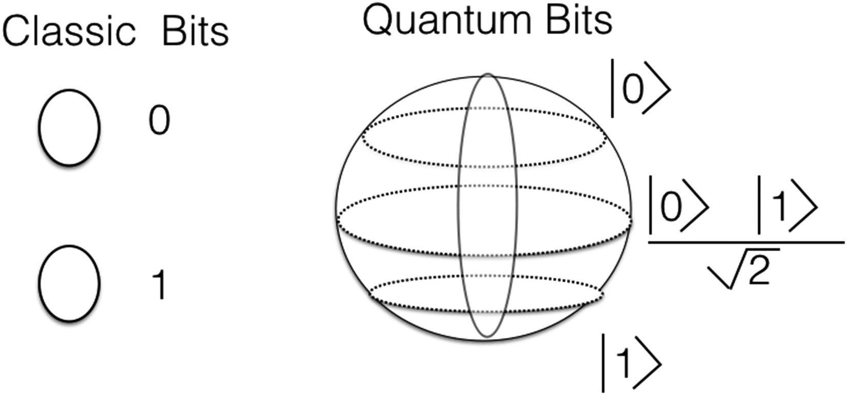
Classic versus quantum bits
Initial Setup
You need to set up Python 3.5 to run the code samples in this chapter. You can download it from https://www.python.org/downloads/release/python-350/.
Single Qubit System
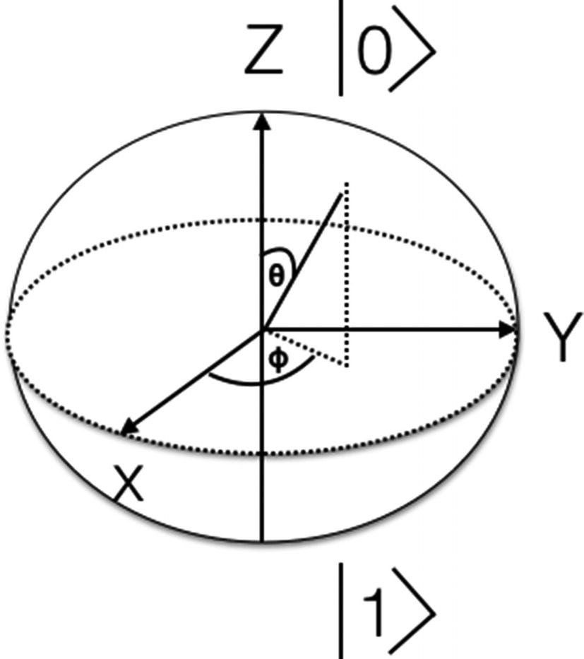
Bloch sphere
Now let’s look at a code sample in Python that demonstrates a single qubit system.
Code Sample
Command for Execution
Output
Multiple Qubit System
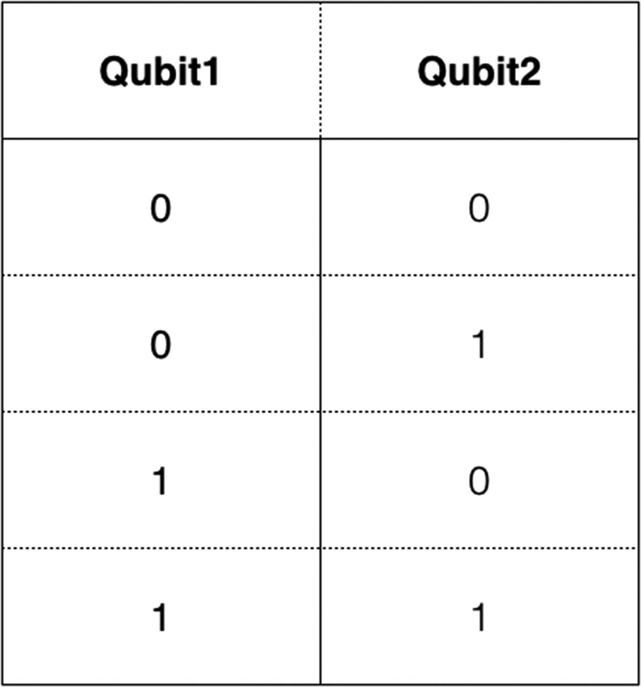
Two qubit system

Three qubit system
The quantum states of the quantum bits in a multiple-qubit system will be a vector with complex coefficients. The real logical state is referred to as observable. The state is measured, and the result is observed. A quantum system will have filters, which are used to identify the quantum state. Different functions are modeled based on the different sets of observables.
A 2 qubit system is specified using the following equation:
q(0) + q(1) = 1
Single quantum bit measurements are used to model 2 qubit measurement operations. A quantum register can be measured partially. The unmeasured leftover is transformed using the identity quantum operation.
Quantum States
A quantum bit exists in 0, 1, or a state between 0 and 1 quantum states. This helps a quantum computer to model a huge set of possibilities through the quantum state. S bits are equivalent to 2S multiple states. The state between 0 and 1 is referred to as quantum superposition. Superposition is modeled as a wave function. A wave function can have infinite states mathematically.
Pure
Mixed
Two quantum states can be mixed with one another to create another quantum state. This is similar to the mixing of matter waves in physics.

Bloch sphere
amp1 and amp2 are called probability amplitudes , which are complex numbers.

Superposition
Figure 3-6 shows the quantum bits in superposition compared to the classical bits’ 0 and 1 states.
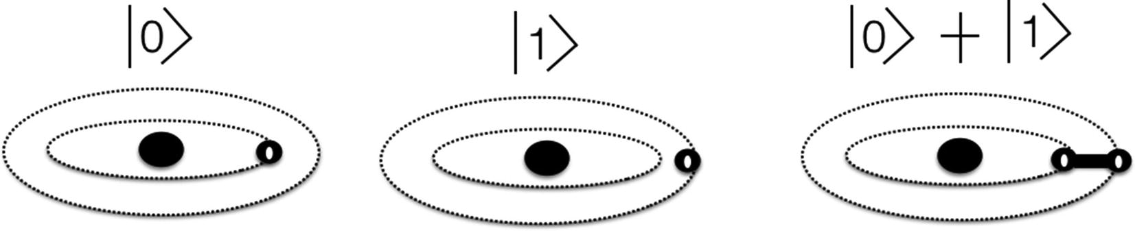
Superposition state of quantum particle
Now let’s look at a code sample in Python to demonstrate the superposition of the quantum bits and states.
Code Sample
Command for Execution
Output
Quantum Protocols
In this section, we look at entanglement and teleportation, which are based on quantum protocols.
Quantum Entanglement
Quantum entanglement is the interaction of multiple quantum particles with each other. The interaction leads to entanglement, and the quantum particles might separate eventually in the space.
This quantum protocol–based phenomenon was observed in 1935 by Albert Einstein, Boris Podolsky, and Nathen Rosen during a quantum mechanical experiment. They wanted to show the logical impossibility of quantum mechanics.
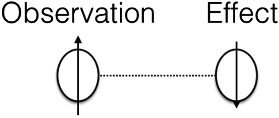
Entanglement
Quantum Teleportation

Teleportation
Quantum Operations

Quantum operations: Bloch sphere
A Bloch sphere is used to represent the quantum operation. The rotation happens around the x-, y-, and z-axes of a unit radius three-dimensional sphere.
Quantum gates are quantum operations using quantum bits. Quantum operations are the building blocks of the quantum circuits. Quantum circuits are the fundamental blocks on which a quantum computer is built.
Let’s start looking at the Hadamard gate first. Hadamard gate is the gate that operates on the base state from |0> to (|0>+|1>)* 1/√2 and |1> to (|0> - |1>)* 1/√2. This gate transformation results in a superposition.
Now, we look at Swap gates. A Swap gate swaps the quantum state of the gate.
Dirac notation is used for writing equations. Paul Dirac was the first person to come up with a unique notation for representing vectors and tensors. This notation is efficient compared to matrices.
An X gate is a quantum equivalent of a NOT gate. A CNOT gate is a controlled-NOT gate. A CNOT gate negates a bit; the control bit is equal to only 1. A Toffoli gate is a controlled-NOT gate, which is a quantum equivalent of an AND gate. Toffoli negates a bit if both control bits are equal to only 1. A Pauli X gate is a quantum operation that rotates a quantum bit over the x-axis with an angle of 180 degrees. A Pauli Z gate is a quantum operation that rotates a quantum bit over the z-axis with an angle of 180 degrees.
Now let’s look at some CNOT, X, Z, and Measure gate implementations to demonstrate the quantum gates. The implementations of a CNOT gate, X gate, Z gate, normalize operation, and Measure gates in Python are shown next.
Code Sample
Command for Execution
Output
Quantum Transformations
Quantum transformations are related to the quantum state transformations using quantum bits. We look at the Kronecker transformation and measure gates in this section.
Kronecker Transformation
A tensor product is used to model a multiquantum bit system. A Kronecker product is a tensor product of vectors and matrices.
A multiquantum state is represented using multiple quantum bits and vectors. The dimensionality of the quantum state increases exponentially with the number of quantum bits in the system.
The tensor product between two quantum states is represented using the symbol ⊗. The multiquantum bit state is shown using Dirac notation as |100>, which is the same as |1> ⊗ |0> ⊗ |0>.
Measure Gate Transformation
where amp1 and amp2 are amplitudes of the quantum bits.
Now let’s look at a code sample in Python to demonstrate a Kronecker transformation in Python.
Code Sample
Command for Execution
Output
Summary
In this chapter, we looked at single and multiple quantum bit systems. Quantum bits system phenomena such as entanglement, superposition, and teleportation were discussed in detail. Finally, the quantum states, gates, and transformations were presented.