Introduction
“A classical computation is like a solo voice—one line of pure tones succeeding each other. A quantum computation is like a symphony—many lines of tones interfering with one another.”
—Seth Lloyd
This chapter gives an overview of a quantum information processing framework. You will see how a quantum information processing framework is applied in real life. Code examples are presented for the quantum algorithms discussed. In addition, this chapter discusses quantum circuits in detail.
Initial Setup
You need to set up Python 3.5 to run the code samples in this chapter. You can download it from https://www.python.org/downloads/release/python-350/.
Quantum Circuits
A quantum circuit is a key part of quantum computing. As we have seen, quantum computing is based on quantum mechanics principles. For example, quantum mechanics principles such as superposition and quantum entanglement are widely used in quantum computing. Quantum bits are the same as the classical bits. The Hilbert state space has the eigenvalues related to the linear superposition. The state values will be |0> and |1>. These eigen states are operated on using unitary operations.
Let’s look at what a Hilbert space is. A Hilbert space is similar to an inner product space of finite-dimensional complex vectors. The inner product of two complex vectors is the same as the inner product of two matrices that represent the vectors. Now let’s see what eigenvalues are. Eigenvalues are complex numbers that satisfy the linear equation B |v > = v|v>. |v> is a nonzero vector, which is the eigenvector with linear operator B.
Let’s look at the superposition principle that was discussed in earlier chapters. The superposition principle in quantum mechanics is related to the states of the quantum system. Let’s say |u> and |v> are the two states of the quantum system. Superposition α|u> + β |v> is a state that is valid if |α|2 + |β|2 = 1. Schrodinger’s equation is another principle from quantum mechanics that is used in quantum computing. The quantum system’s state evolves with time. The time evolution is explained mathematically by Schrodinger’s equation.

Quantum circuit
The quantum circuit model is based on the quantum entanglement of quantum bits. Quantum entanglement has no classical equivalent. The superposition principle is used in quantum computers to save data in exponential size compared to classical computers. Classical computers using M bits can save one out of the 2M combinations. Quantum computers can save 2M combinations of information. Let’s see what quantum entanglement is. We discussed quantum entanglement in the initial chapters. Entanglement is related to a pair of entangled particles whose state is dependent on each other. This phenomenon is observed when they are separated by huge distances.
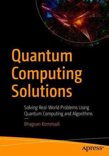
Quantum circuits are used to create a quantum computer. The circuit consists of wires and quantum gates. Quantum logic gates are based on either a quantum bit or multiple quantum bit gates. These gates are reversible. Quantum gates are used to transmit and modify the information.
CNOT gate circuit
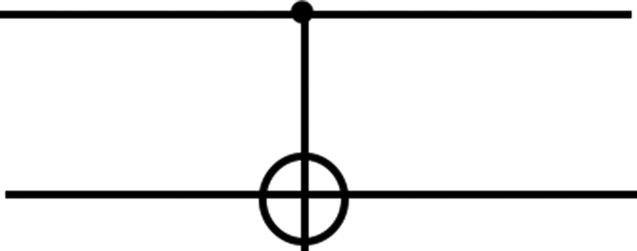
CNOT gate circuit in matrix form
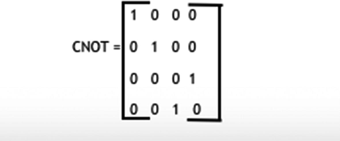
Controlled-U gate circuit
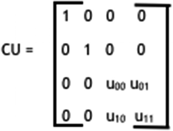
Controlled-U gate circuit matrix
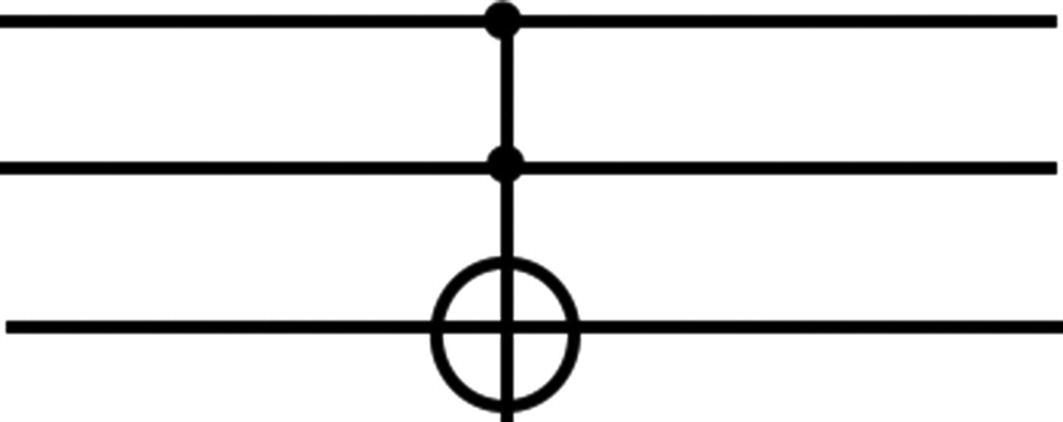
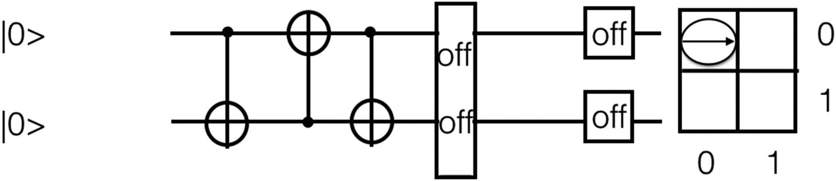
Toffoli gate circuit
A Toffoli gate has an input of 3 bits and an output of 3 bits. Out of the three input bits, two of them are control bits, and the third bit is a target bit. If control bits have a value of 1, the target bit is flipped. If the control bits do not have a value of 1, the control bits are not changed.
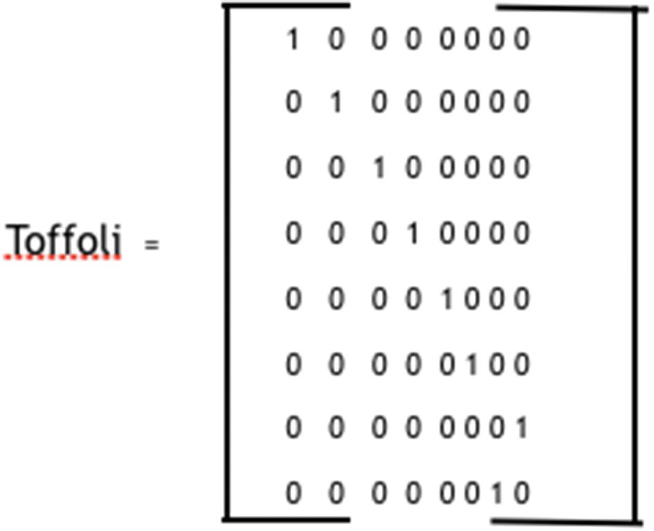
Toffoli gate circuit matrix
After looking at the different types of quantum circuits, the last step in the quantum circuit model is the measurement projected on the computational scale. This step is not reversible. There are two types of measurement: deferred and implicit. The deferred measurement method allows changing the quantum operations to the classical equivalents. In this method, a measurement can be sent from the middle stage to the end of the circuit. In the implicit measurement method, quantum bits that are not measured can be measured implicitly. In this method, generality loss does not happen.
A quantum circuit has reversible changes to a mechanical analog, which is a quantum register.
Quantum Communication
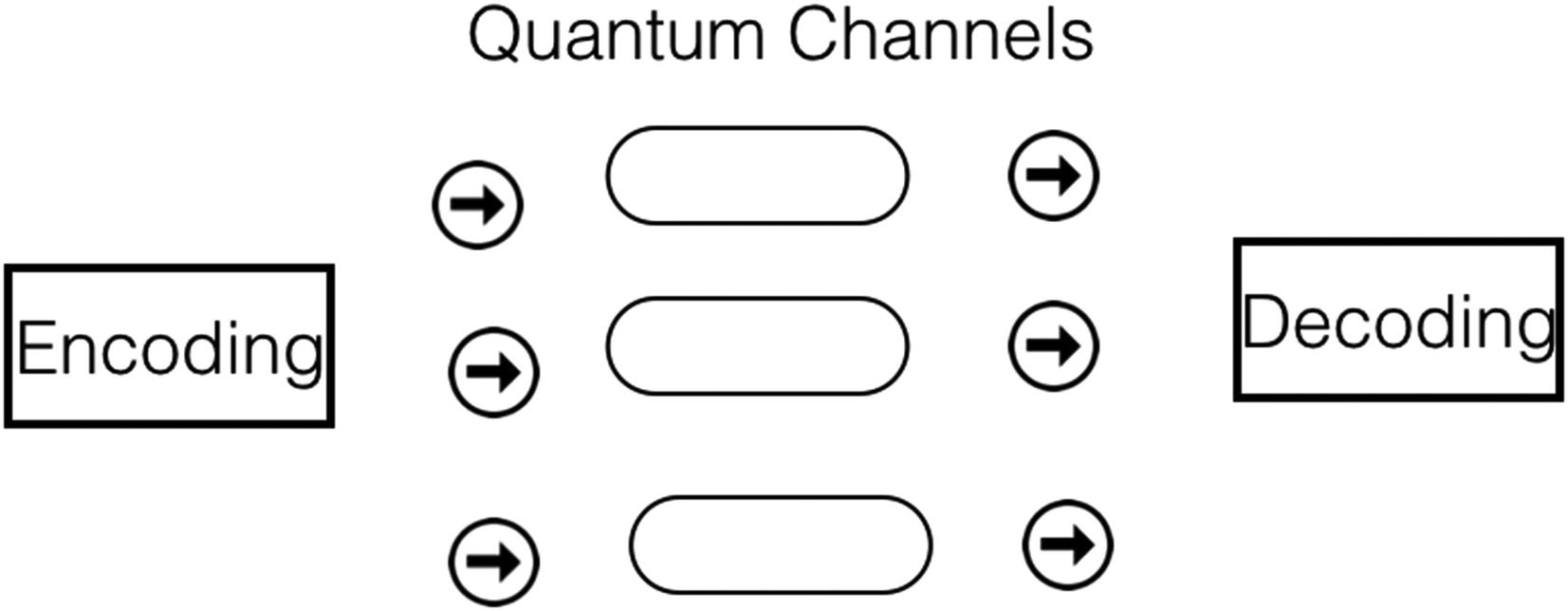
Quantum communication
In superdense coding, classical information bits are transferred from the source to the destination. In quantum teleportation, quantum bits are transferred by using the communication channel between two classical bits.
The superdense protocol has an instruction set and the output results. The protocol is valid if it generates the expected output. The superdense protocol is based on quantum entanglement. Quantum entanglement occurs when a single common source can produce multiple quantum systems. The state of the quantum systems does not follow Bell inequality rules. The systems that are entangled impact each other even if they are separated by huge distances.
We have looked at the superdense quantum communication protocol; the other protocols are the continuous variable, satellite, and linear optics quantum communication protocols. The electric field of the incident light is measured using a homodyne detector. The measurement results in a continuous value. Continuous variable quantum communication is based on the homodyne detector measurement outcome. The satellite communication protocol is based on ground-to-satellite and satellite-to-satellite communication channels. The linear optical quantum communication protocol is based on optical fiber–based communication channels.
Quantum Noise
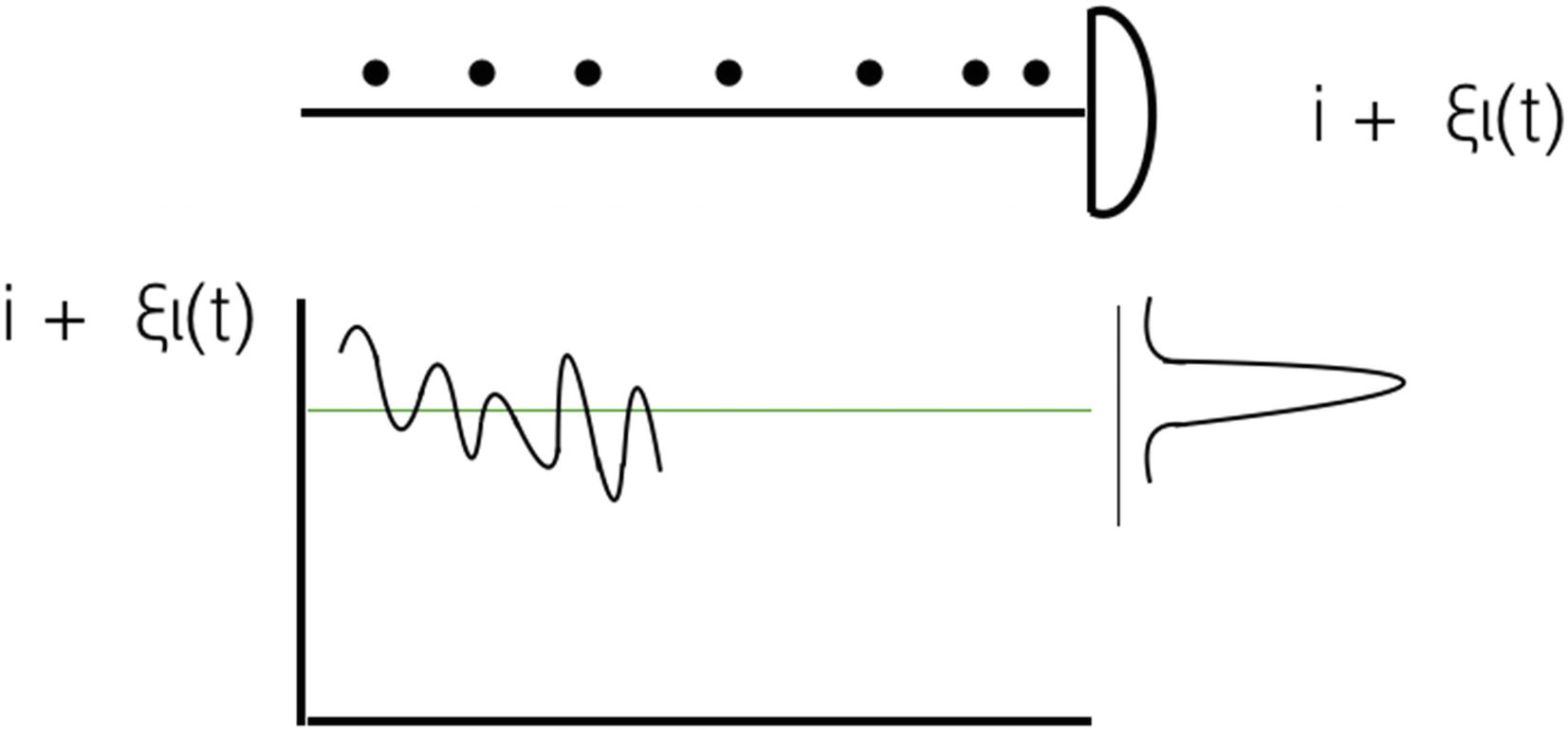
Quantum noise
H.B.Callen and T.A.Welton represented the spectral density in mathematical equations. Roger H.Koch measured the spectral entities of the quantum noise experimentally first. Spectral density is related to the signal periodograms of time segments. Mathematically, Fourier analysis is a good method to measure spectral density by breaking down the function to a set of periodograms. A periodogram is a time period series in mathematics.
Quantum noise happens because of signal changes in an electric circuit. The signal changes occur because of the electron’s discrete character.
Quantum Error Correction
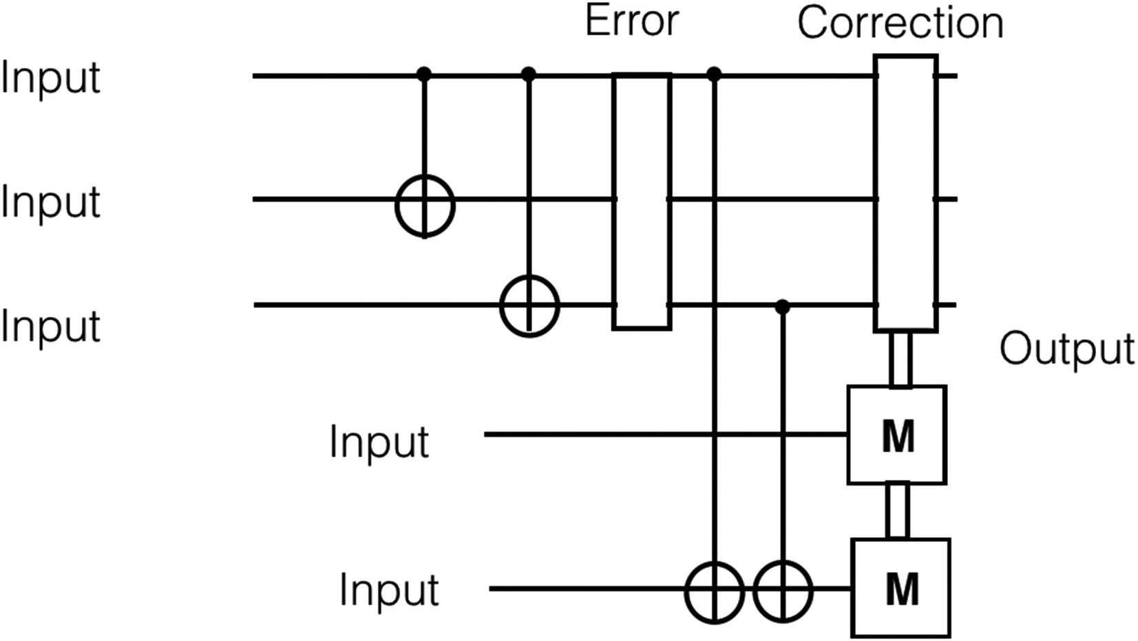
Quantum error correction
Let’s look at classical error correction techniques such as coding. Coding is related to data cloning. This technique is not helpful for quantum error correction because of the no-cloning principle. The no-cloning principle states that a quantum state that is not known cannot be copied exactly. Quantum error correction does not allow a huge number of copies. Errors cannot be prevented by using direct measurement because quantum superposition fails. Quantum errors can happen due to quantum bit flip, phase shift, and continuous errors.
Now let’s look at how to fix quantum errors. Coherent techniques help to bring down the control errors. The errors due to decoherence are time dependent. Modeling the errors helps to measure the errors, and positive operator–valued measures are used to measure the errors. Tracing the lost quantum bit is another way to model the quantum bit loss and removal. Correction is done by validating the presence of the quantum bit in the system first. Quantum bits are lost due to controls that are significant. The Shor code protocol designed by Peter Shor helps in identifying and fixing the errors from a quantum bit.
Let’s now look at the Shor code protocol. The Shor code is a group of three quantum bit phase flip and bit flip codes. This quantum code helps to guard against the error impact on a quantum bit. Quantum states are operated by the unitary operation to result in a quantum error correction–based code. This result will be part of the subspace D of a bigger Hilbert space. A Hilbert space is an inner product of finite-dimensional complex vectors.
Limitations of Quantum Computing
Let’s look at the limitations of quantum computing before we look at different quantum algorithms. Quantum computers are prone to errors and problems due to the environment. Decoherence happens because of the collapse of the state function due to the measurement of state for a quantum bit. Decoherence causes the errors in the computation. The quantum bits count impacts the decoherence probability exponentially. Decoherence occurs because of the quantum bit flip, spontaneous symmetric breaking, and phase flip coding protocols. Quantum bit flip code flips the quantum bit based on a probability. The symmetric breaking protocol is based on a symmetry group F if an F transformation on the quantum system can be achieved by operating transformations on the quantum subsystems. Quantum bit phase flip code is based on the flip of the phase based on a probability.
Small errors can be removed by using error correction protocols in classical computation. In quantum computation, small errors cannot be fixed. Quantum systems are entangled to the environment, and hence the error is induced before the computation begins. Initialization of the quantum bit induces the errors due to unitary transformations.
Quantum Algorithms
Algorithms are used in computation and data processing. The real-life situations are modeled and solved using heuristics and methods. An algorithm consists of a set of commands to execute a task. Quantum algorithms help in providing solutions to complex problems that cannot be solved by classical computers.
Quantum programming languages help to create quantum software with quantum algorithms. A quantum algorithm consists of steps such as encoding the quantum data to quantum bits, a unitary quantum gates chain operating on the quantum bits, and terminating after measuring the quantum bits. A unitary quantum gate is similar to a unitary matrix that operates on the quantum bits. A unitary matrix inverse will be equal to its conjugate transpose.
Quantum computing is based on quantum mechanical properties such as superposition and entanglement. Specifically, quantum algorithms use these principles.
The word algorithm word originates from the word algebra. It is named after Arabian mathematician Al Khwarizmi.
Let’s look at some quantum algorithms, starting with the Deutsch–Jozsa algorithm.
Deutsch–Jozsa Algorithm
Oracle function
This algorithm uses a black-box (Oracle) function that takes as input the binary values and gives either 0 or 1 as output. The method finds whether the function g used is constant or balanced.
In the next sections, we discuss the algorithm implementation. To start with, let’s look at the quantum register. The quantum register has a constructor and GetMeasure and ApplyOperation methods. The GetMeasure method computes the quantum states and probabilities. The ApplyOperation method updates the class instance variable data to the product of the input gate matrix and data instance.
Code Sample
Now let’s look at the quantum gate implementation. It has a constructor, matrix multiplication, and power methods. The matrix multiplication method operates on the input data and the instance data to return a Kronecker product. The power method takes the input to return the quantum gate.
The I, H, X, Y, and Z gates are initialized in this class. The U_Quantum_Gate gate method creates a quantum gate based on the input parameters.
Code Sample
Functions g1_func, g2_func, g3_func, and g4_func are shown in the code sample. g1_func takes v and returns v. g2_func takes v as an input value and returns value 1. g3_func takes v and w as input values and returns the binary XOR of v and w. g4_func takes v, w, and x as input values and returns a zero value. The CheckIfConstant method takes the input function and an integer to validate whether the function is a constant or balanced function.
Code Sample
Command for Execution
Output
A balanced Boolean function yields output of Booleans 0s equal to 1s. A constant function has an output value as a constant.
Simon’s Algorithm
Now let’s look at Simon’s quantum algorithm. This algorithm helps in identifying a black-box function h(x), where h(x) = h(y) and x= y ⊕ t. Note that t ∈ {0, 1}n and ⊕ represents bitwise addition based on module 2. The goal of the algorithm is to find that by using h. This quantum algorithm performs exponentially better than the classical equivalent. This algorithm inspired Shor to come up with Shor’s algorithm.
Let’s look at the Python code implementation of this algorithm.
The RetrieveOnetoOneMap method takes the input mask as a parameter and returns the output, which is a bitmap function. The RetrieveValidTwoToOneMap method takes input parameters such as search mask and random seed. It returns output that is a two-to-one mapping function.
Code Sample
The Simons_Algorithm class is used to find the black-box function to satisfy a set of values. It has a constructor and the following methods: RetrieveSimonCircuit, CalculateUnitaryOracleMatrix, RetrieveBitMaskRetrieveSampleIndependentBits, RetrieveInverseMaskEquation, AppendToDictofIndepBits, RetrieveMissingMsbVector, and CheckValidMaskIfCorrect. The RetrieveSimonCircuit method takes as input the quantum bits and returns the output, which is the quantum circuit.
The CalculateUnitaryOracleMatrix method of the Simons_Algorithm class takes the input map of bit strings. The output will be a dense matrix, which is a permutation of the values from the dictionary. The RetrieveBitMask method of the Simons_Algorithm class takes as input the quantum computer and bit strings. The output is a bit string map.
The RetrieveSampleIndependentBits method takes as input the quantum computer and bit strings. The independent bit vectors are updated with the bit strings. The RetrieveInverse mask equation method creates the bit mask based on the input function. The AppendToDictofIndepBits method takes as input an array. This method adds to the dictionary of the independent vectors. The RetrieveMissingMsbVector method searches the provenance value in the set of independent bit vectors. The method modifies the collection by adding the unit vector. The CheckValidMaskIfCorrect method validates the given mask if it is correct.
Command for Execution
Output
Shor’s Algorithm
Peter Shor was the first to come up with a quantum algorithm for the factorization of integers in 1994. Shor’s algorithm performs in polynomial time to factor an integer M. The order of performance is O(logN). This outperforms the classical equivalent. In addition, this algorithm has the potential to break the RSA cryptographic method.
The algorithm takes a number M and finds an integer q between 1 and M, which divides M. The algorithm has two steps: the reduction of factoring to order the finding method and the order finding technique.
If gcd(b,M) != 1, there are nontrivial factors for M, and the problem is solved.
- If gcd(b,M) == 1 , find the period of g(x) = ax mod M to find r for which g(x+r) = g(x) (this is step 1).
If r is odd, go back to step 1.
If ar/2 = -1 (mod M), go back to step 1.
gcd(ar/2 +- 1, M) is a nontrivial factor of M. The problem is solved.
Now let’s look at the quantum algorithm. The quantum circuit for the algorithm is based on M and a in g(x) = ax mod M: Given M, Q= 2q and Q/r > M. The input and output quantum bits have superpositions of values from 0 to Q-1, and they have q quantum bits each. The g(x) function is used to transform the states of the quantum bits. The final state will be a superposition of multiple Q states, which will be Q^2 states.
Let’s look at the Shor’s algorithm implementation in Python.
Shor’s algorithm is used for prime factorization. The QuantumMap class has the properties of state and amplitude. QuantumEntanglement has the properties of amplitude, register, and entangled. The UpdateEntangled method of the QuantumEntanglement class takes input parameters such as state and amplitude. The RetrieveEntangles method returns the list of entangled states.
Code Sample
The QuantumRecord class has numBits, numStates, an entangled list, and a states array. The SetPropagate property of the QuantumRecord class takes fromRegister as the parameter and sets propagate on the register. The UpdateMap method takes such inputs as toRegister, mapping, and propagate parameters. This method sets the normalized tensorX and tensorY lists. The FindMeasure method of the QuantumRecord class returns the output, which is the final X state. The RetrieveEntangles method takes as input the register and returns the output, which is the entangled state value. The RetrieveAmplitudes method returns the output, which is the amplitudes array of quantum states.
Code Sample
The FindListEntangles method prints the list of entangles. The FindListAmplitudes method prints the values of the amplitudes of the register. The InvokeHadamard method takes input such as lambda x and the quantum bit. The codomain array is returned as the output. The InvokeQModExp method takes the input parameters aval, exponent expval, and the modval operator value. The state is calculated using the method InvokeModExp.
The InvokeQft method takes inputs such as parameters x and the quantum bit Q. The quantum mapping of the state and amplitude is returned by the method InvokeQft. The FindPeriod method takes the inputs a and N. The period r for the function is returned as output from this method.
The ExecuteShors method takes inputs such as N, attempts, neighborhood, and numPeriods as parameters. This method applies Shor’s algorithm to find the prime factors of a given number N.
Code Sample
Command for Execution
Output
Grover’s Algorithm
Grover’s algorithm is used for searching a database. The search algorithm can find an entry in a database of M entries with O (√N) time and O(logN) space. This method was found by Lov Grover in 1996. He found that his method gave a quadratic speedup compared to other quantum algorithms. In addition, Grover’s method gives exponential speed over the classical equivalents.
Grover’s algorithm inverts a function. Let’s say y = g(x). Grover’s algorithm finds x when y is given as input. Searching for a value of y in the database is similar to finding a match of x. It is popular when solving NP-hard problems by using exhaustive search over a possible set of solutions. You can use Grover’s algorithm to search for a phone number in a phone book of M entries in √ M steps.
- 1.
Initialize the system to the state.
- 2.
Execute the Grover iteration r(M) ties.
- 3.
Measure the amplitude Ω.
- 4.
From Ωw (result), find w.
Let’s look at the implementation of Grover’s algorithm in Python.
Grover’s search algorithm searches the target value of a group by computing the mean amplitude and Grover’s amplitude. The plot of the graph is computed from the amplitudes derived from Grover’s algorithm. The plot presents the target value with the highest amplitude. The ApplyOracleFunction method takes input x and returns the output as the hex digest of x. ApplyGrover’s algorithm takes as input the target, objects, nvalue, and rounds. The amplitude is returned as the output.
The target of the algorithm is to search for 9 in the group of string objects {'14', '5', '13', '7','9','11','97'}. The amplitude is searched from the dictionary (group of string objects) based on the value 1/ square root of the length of the set (9).
Code Sample
Command for Execution
Output
Quantum Subroutines
Quantum computer simulators are built to simulate a quantum computer of size n quantum bits. Quantum computer simulation packages are now available to write software related to quantum computing. The packages are like black boxes that abstract the methods and techniques of quantum algorithms. The quantum Fourier transform, QPhase, and matrix inversion subroutines are available in the packages to help solve complex problems in real life.
The software packages are Project Q, IBM Quantum Experience, PennyLane, QuidPro, Liquid, etc. Quantum circuits can be simulated using the packages for analysis and computation.
The applications are developed using the quantum subroutine packages for quantum and classical algorithms. The code is compiled, and the input files are used for quantum algorithms to execute the algorithm. Quantum circuits are modeled using the subroutine API packages. The quantum circuits have a set of control gates, and measurements are performed on the simulated quantum circuits.
Execution of the quantum algorithms takes place using the group of quantum circuits that represent and model the real-life problem. The postprocessing of the results is performed for analysis purposes.
Summary
In this chapter, we looked at quantum circuits, quantum communication, quantum noise, quantum error correction, and the limitations of quantum computing. Quantum algorithms such as Deutsch–Jozsa, Simon, Shor’s, and Grover’s were discussed in detail. Quantum subroutines and algorithms were also presented with examples.