
The AES block cipher is the same as the Rijndael algorithm but with a fixed block size of 128 bits (see Chapter 12). In IEEE 802.11i RSN, a further simplification is made by restricting the key size as well as the block size to 128 bits. The following description relates only to the RSN version.
You can think of the encryption of the block of data as a sort of production process in which various operations are applied repeatedly until the finished product, the ciphertext, is produced. A medieval blacksmith made a sword by starting with a strip of iron and repeatedly heating it, hammering it, adding impurities, folding it, and quenching it in cold water. By folding the metal ten times, the sword ended up with a thousand fine layers. In AES the data is the raw material loaded into a state array. The state array is processed through ten rounds of manipulation, after which it is unloaded to form the resulting encrypted block of data. At each stage of the process, the state is combined with a different round key, each of which is created and derived from the cipher key.
Although this sounds like a lot of work, one of the key advantages of the Rijndael algorithm is that it uses only simple operations such as shift, exclusive OR, and table substitution. Many encryption approaches require multiplication operations that are very expensive to implement. Rijndael uses finite field byte multiplication, a special operation that can be simplified down to a few logical operations or lookups in a 256-byte table. This appendix begins with an overview of finite field arithmetic. If you are just interested in the encryption steps for AES, skip to the next section.
When you were six years old, you probably spent quite a bit of time reciting multiplication tables and doing long additions and multiplications. You might have found it hard to remember to pass the carry from one column of digits to the next in an addition, but you did it because the teacher said, “This is the way the world works.” Now you encounter finite field arithmetic, which has a different set of rules and, on first inspection, sounds like it came from outer space. Finite field arithmetic is important in cryptography and is the basis of the familiar cyclic redundancy check (CRC) used to detect errors in data packets.
Conventional arithmetic operates on an infinite range of values, even if you limit it to positive integers. However, if your entire universe is defined by a single byte, you have only 256 values to deal with. What often happens is that normal arithmetic is applied to byte values and any overflows or underflows during the conventional arithmetic are discarded. This works for many types of calculations, but in some sense discarding the carry violates the rules of conventional arithmetic. Your primary school teacher didn't talk about number universes that had only 256 values. Finite field arithmetic is defined specifically to handle such finite number universes. The rules apply to cases like single byte arithmetic so, in some sense, it is more valid than the familiar arithmetic. But let's not get too philosophical here; this type of arithmetic enables some good tricks and allows some neat shortcuts in the computations. This section is not intended to be a rigorous description of finite field mathematics; and if you are a pure mathematician, you probably won't like it. However, we do introduce the basics and explain why some of the computations used in cryptography look a little weird.
For our application, we are interested only in finite fields that can be represented by binary numbers. For purposes of finite field arithmetic, we can represent a binary number by polynomials of the form:
The value of x is not important as it is only the coefficients a(n) that we are interested in. However if the coefficients have the value 0 or 1 and x represents the value 2, then the value of the polynomial, computed using conventional arithmetic, corresponds to the binary value.
Each of the coefficients corresponds to one bit of a binary number. So, for example, the 8-bit value 10010111 would be written as:
or more simply:
Treating the numbers as polynomials leads to some interesting and different behavior when you are performing arithmetic operations. This is okay, providing such treatment still follows some basic rules such as:
if A + B = C then A = B – C
and if A × B = C then A = C÷B
In the following sections we look at the main operations in turn.
When you add two polynomials, each term is added independently; there is no concept of a carry from one term to another. For example, in conventional arithmetic
In our binary representation, the coefficients can be only 0 or 1. The value 2 is not possible. Therefore, we have the rule that, when adding the coefficients, the following addition rule applies:
0 + 0 = 0
0 + 1 = 1
1 + 0 = 1
1 + 1 = 0 (there is no carry)
By a useful coincidence, this is the same result as what you get when you perform an exclusive OR operation, which is easier for digital logic than a binary addition.
Using our binary rules, the addition of the two polynomials in equation A.4 is:
This corresponds to the binary computation:

Notice how the addition has now been entirely replaced by the exclusive OR operation. Addition of 2 bytes under these rules is really an XOR operation, and addition cannot have a result bigger than 1 byte, which is consistent with our 1-byte universe.
The same logic that made addition become XOR also applies to subtraction. Suppose we want to subtract the two polynomials in (A.4). In conventional arithmetic the result would be:
The coefficient of the x term is –1. There is no –1 value in a single binary digit. The subtraction table for two binary digits is:
1 – 1 = 0
1 – 0 = 1
0 – 1 = 1 (there is no borrow)
0 – 0 = 0
Once again this is the same as the XOR operation so that the binary subtraction takes the form:

Surprising but true—in this byte arithmetic universe addition and subtraction become the same operation and are replaced by the exclusive OR operation. Notice also how this new arithmetic also obeys the rule that if A + B = C, then A = B – C.
Multiplication deviates even more from conventional arithmetic because of the way polynomials multiply together. The basic rule for multiplying two polynomials is to multiply all the terms together and then add terms of similar order (in other words, the same power of x). Here is a simple example in normal mathematics:
By now you might guess that in our binary universe the x4 term will disappear, leading to the result:

So far this looks straightforward enough and, by following the good old school long multiplication rules, we can work out the multiplications using only shift and XOR operations:
Multiplying by x2 is the same as shifting left by two places because:
This means that the long multiplication can be done using the accumulate row method as follows:

Notice how the intermediate rows are just the first value shifted and the result is just the XOR of the rows. Great! Now we have a really efficient way to do addition, subtraction, and multiplication by using this polynomial-based arithmetic. However, there is a snag that we discuss after looking at division.
Division works by the shift and subtract method familiar under the name long division. Of course, in our case the subtraction is done using an XOR operation. An example is shown here and should be fairly self-explanatory:

This is the reverse of the multiplication shown in the previous section. Gratifyingly, we get back to the result before the multiplication, showing that our arithmetic satisfies the rules that if A × B = C, then B = C ÷ A.
Now comes the hard part. Not hard to implement but hard to understand. When we did addition and subtraction, it was not possible for the result to overflow. The result always fitted into a byte. However, based on our long multiplication approach, it is clearly possible that the result of multiplying two 8-bit numbers could be more than 8 bits long. Such an overflow is not allowed to exist in our finite field of 256 values, so what has gone wrong?
Let's go back to ordinary numbers instead of polynomials for a moment. Let's define a finite field that comprises seven digits {0, 1, 2, 3, 4, 5, 6}. We will define addition and multiplication to be the conventional operations except that the result “rolls over” from 6 back to 0. So if we add 1 to 6, we get 0. If we multiply 2 by 4, we get 1 (2 * 4 = 4 + 4 = 6 + 2 = 1—work it out). We can make an addition table, as shown in Table A.1. Taking any two numbers from the top row and left column, the sum is found in the intersection of the row and columns.
In a similar way we can define a multiplication table, as shown in Table A.2. Here the product value is in the intersection of each row and column. These tables can be used for subtraction and division as well. To work out the value of m/n, you go to the nth column, find the entry m in the column, and the answer is the row number. For example, to compute 6/3, go to the third column and find the value 6, then look to the left to see the answer 6/3 = 2. Note that this rule does not work if you try to divide by 0; try it and you'll see the problem. As with conventional arithmetic, dividing by 0 is undefined.
These tables show that it is possible to define a finite number universe with familiar and useful arithmetic operations that really work. However, this approach does not work in all cases. Suppose we want a universe with six numbers: {0, 1, 2, 3, 4, 5}. Applying the “roll over rule” whereby 5 + 1 = 0, the addition and multiplication tables come out as shown in Tables A.3 and A.4.
Look at column 2 of the multiplication table. 0 appears twice. Numbers 1, 3, 5 don't appear at all! Column 3 only has the values 0 and 3. What this means is that it is impossible to do meaningful division in this number universe. The problem is that there are six numbers and both 2 and 3 are factors of 6. This means that 2 * 3 = 0 and also 2 * 0 = 0.
Because of this factoring problem, this type of finite number universe can only have all four arithmetic operations (+, –, *, ÷) if the number of values in the universe is a prime number. It works when there are seven values because seven is a prime number. It doesn't work with eight, nine, or ten values, but it works with eleven values and so on.
If we return to our polynomial representation, a similar rule applies. The finite field should be bounded by a polynomial that is irreducible. A polynomial is reducible if it can be factored. For example (x2 + 1) is reducible because:
To make our finite field arithmetic work, we need a finite field that is bounded by an irreducible polynomial and has 256 elements. Such a field can be created and is called a Galois Field, denoted by GF(256). We will not present the theory behind how a Galois Field is created. However, it has the property that it has 2n entries and the entries are derived from, and bounded by, an irreducible polynomial. For GF(256), that polynomial is:
This corresponds to the binary value 100011011 or hexadecimal 11B.
Let's remind ourselves of why we digressed to discuss the Galois Field. The problem was that multiplication according to the rules we had defined caused undefined results due to overflows. The question was how these should be handled and avoided? The answer lies in treating the possible 256 values as members of the GF(256) field. This field is limited by the irreducible polynomial that defines our GF(256). We can think of the rules of multiplication in the same way as shown in Table A.2. In that case the result wraps around the prime number that defines the number of elements in the field; in Table A.2 this prime number is 7. In conventional arithmetic, we would say that the result is the remainder after dividing by 7 or that the result is computed modulo 7.
In Table A.2, a multiplication can be computed as follows:
Result = (A x B) mod 7.
or
Result = Remainder((A x B) / 7)
Example: 6 * 6 = 36 mod 7 = Remainder(36/7) = 1
The same rule is now applied to our byte computations in the GF(256) field:
Result = (A x B) mod x8 + x4 + x3 + x1 + 1 (the irreducible polynomial)
or
Result = Remainder( (A x B) / (x8 + x4 + x3 + x1 + 1) )
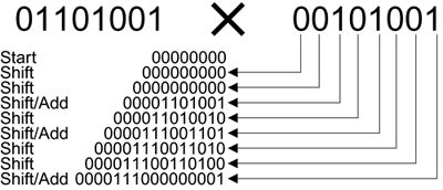
Lets see how this works in practice. We saw in (A.11) the result of a multiplication that did not overflow outside the byte value. Let's take an example that clearly does want to overflow:
01101001 * 00101001
Using the accumulate row approach:

The intermediate result in (A.15) is 12 bits long—we need to reduce it by wrapping around the irreducible polynomial. To do this, we need to divide by our irreducible polynomial and take the remainder:

So the remainder after removing the overflow is 10000011. In other words, in our finite field:
01101001 * 00101001 = 10000011
All values are within our single byte space. Hooray! However, although it still uses only shift and XOR, the computation now seems rather complicated and long-winded. We had to do both long multiplication and long division to get the result. There is a good trick we can use to simplify the computation, however. If we look at the accumulate row approach to multiplication, each intermediate row represents the first multiplier shifted left to correspond to a bit in the second multiplier. After this, all the rows are added together and the result is taken modulus our field polynomial 100011011. However, rather than waiting until all the rows are accumulated before adding together, you can shift and add 1 bit at a time as the computation proceeds. Let's look at the previous multiplication, 01101001 * 00101001, done in this way. The sequence of events is shown in Figure A.1. The process for computing A x B is as follows:
Start with an accumulator value of 0.
Take each bit of B in turn, starting with the most significant bit.
For each bit, first multiply the accumulator by 2 (shift left).
If the bit is 1, add the value of A to the accumulator.
The final value of the accumulator is the answer.
Figure A.1 shows the computation for the same example we used earlier (A.15) and you can see that the result is the same—this is good. In the previous example we reduced the result of (A.15) to be within range by dividing by the value 100011101 and taking the remainder. This gave the result shown in (A.16). However, if we use the shift and add approach, there is another way to do the reduction that is easier than performing this long division. Note that the shift and add method requires that the accumulator be shifted left at each stage. This left shift is the same as multiplying by two. The simplification is to reduce the value within range after each shift rather than waiting until the end.
You might think that means more divisions rather than fewer. However, consider the result of the computation 2 * A. If the most significant bit of A is 0, we know that there cannot be an overflow so the result will already be in range. If the most significant bit is 1, we know that there will be an overflow. Because we know the result overflows, it needs to be reduced to get back to a byte value. We also know that the range of possible values after the shift will be 100000000 to 111111110. This means that the result of dividing by 100011011 must always be 1 and the remainder will be the result we want. Because we know the result of the division is 1, we can get that wanted remainder simply by subtracting 100011011 from the shifted value. So now we have a simple rule for computing 2 * A:
In the second case, the XOR accomplished the “subtract 100011011” operation for the byte value.
Now we have a long multiplication rule that works for all cases. The shift operation in Figure A.8 is replaced by the formula in (A.17). Each intermediate step as well as the final result is guaranteed to be within the GF(256) field; in other words, the result of the multiplication is always a single byte. The long multiplication has been achieved by a short sequence of XOR operations and shifts that are easily implemented in digital systems.
This section introduces mathematics that may be unfamiliar to you. The arguments seem logical, but you may be left feeling that the operations are puzzling and nonintuitive. However, the benefit of this type of mathematics is an amazing simplification in the way multiplication is implemented. It makes the design and implementation of encryption systems, which often rely on many multiplications, much more practical in the real world.
The encryption process uses a set of specially derived keys called round keys. These are applied, along with other operations, on an array of data that holds exactly one block of data—the data to be encrypted. This array we call the state array.
You take the following steps to encrypt a 128-bit block:
Derive the set of round keys from the cipher key.
Initialize the state array with the block data (plaintext).
Add the initial round key to the starting state array.
Perform nine rounds of state manipulation.
Perform the tenth and final round of state manipulation.
Copy the final state array out as the encrypted data (ciphertext).
The reason that the rounds have been listed as “nine followed by a final tenth round” is because the tenth round involves a slightly different manipulation from the others.
The block to be encrypted is just a sequence of 128 bits. AES works with byte quantities so we first convert the 128 bits into 16 bytes. We say “convert,” but, in reality, it is almost certainly stored this way already. Operations in RSN/AES are performed on a two-dimensional byte array of four rows and four columns. At the start of the encryption, the 16 bytes of data, numbered D0 – D15, are loaded into the array as shown in Table A.5.
Each round of the encryption process requires a series of steps to alter the state array. These steps involve four types of operations called:
SubBytes
ShiftRows
MixColumns
XorRoundKey
The details of these operations are described shortly, but first we need to look in more detail at the generation of the Round Keys, so called because there is a different one for each round in the process.
The cipher key used for encryption is 128 bits long. Where this key comes from is not important here; refer to Chapter 10 on key hierarchy and how the temporal encryption keys are produced. The cipher key is already the result of many hashing and cryptographic transformations and, by the time it arrives at the AES block encryption, it is far removed from the secret master key held by the authentication server. Now, finally, it is used to generate a set of eleven 128-bit round keys that will be combined with the data during encryption. Although there are ten rounds, eleven keys are needed because one extra key is added to the initial state array before the rounds start. The best way to view these keys is an array of eleven 16-byte values, each made up of four 32-bit words, as shown in Table A.6.
To start with, the first round key Rkey0 is simply initialized to the value of the cipher key (that is the secret key delivered through the key hierarchy). Each of the remaining ten keys is derived from this as follows.
Table A.6. Round Key Array
32 bits | 32 bits | 32 bits | 32 bits | |
|---|---|---|---|---|
Rkey0 | W0 | W1 | W2 | W3 |
Rkey1 | W0 | W1 | W2 | W3 |
Rkey2 | W0 | W1 | W2 | W3 |
Rkey3 | W0 | W1 | W2 | W3 |
Rkey4 | W0 | W1 | W2 | W3 |
Rkey5 | W0 | W1 | W2 | W3 |
Rkey6 | W0 | W1 | W2 | W3 |
Rkey7 | W0 | W1 | W2 | W3 |
Rkey8 | W0 | W1 | W2 | W3 |
Rkey9 | W0 | W1 | W2 | W3 |
Rkey10 | W0 | W1 | W2 | W3 |
For each of the round keys Rkey1 to Rkey10, words W1, W2, W3 are computed as the sum[1] of the corresponding word in the previous round key and the preceding word in the current round key. For example, using XOR for addition:
Rkey5: W1 = Rkey4:W1 XOR Rkey5:W0,
Rkey8: W3 = Rkey7:W3 XOR Rkey8:W2 and so on.
The rule for the value of W0 is a little more complicated to describe, although still simple to compute. For each round key Rkey1 to Rkey10, the value of W0 is the sum of three 32-bit values:
The value of W0 from the previous round key
The value of W3 from the previous round key, rotated right by 8 bits
A special value from a table called Rcon
Thus, we write:
Rkeyi:W0 = Rkey(i-1):W0 XOR (Rkey(i-1):W3 >>> 8) XOR Rcon[i]
where W >>> 8 means rotate right 8—for example (in hexadecimal) 1234 becomes 4123 and Rcon[i] is an entry in Table A.7.
There is a good reason why the sequence of this table suddenly breaks off from 128 to 27. It is because of the way finite fields overflow, as described in the previous section.
Although the algorithm for deriving the round keys seems rather complicated, you will notice that no difficult computations have been performed and it is not at all computationally intensive. Also note that, after the first, each key is generated sequentially and based on the previous one. This means that it is possible to generate each round key just in time before it is needed in the encryption computation. Alternatively, if there is plenty of memory, they can be derived once at the start and stored for use with each subsequent AES block.
Having described how the round keys are derived, we can now return to the operations used in computing each round. Earlier we mentioned that four operations are required called:
SubBytes
ShiftRows
MixColumns
XorRoundKey
Each one of these operations is applied to the current state array and produces a new version of the state array. In all but the rarest cases, the state array is changed by the operation. The details of each operation are given shortly.
In the first nine rounds of the process, the four operations are performed in the order listed. In the last (tenth) round, the MixColumns operation is not performed and only the SubBytes, ShiftRows, and XorRoundKey operations are done.
This operation is a simple substitution that converts every byte into a different value. AES defines a table of 256 values for the substitution. You work through the 16 bytes of the state array, use each byte as an index into the 256-byte substitution table, and replace the byte with the value from the substitution table. Because all possible 256 byte values are present in the table, you end up with a totally new result in the state array, which can be restored to its original contents using an inverse substitution table. The contents of the substitution table are not arbitrary; the entries are computed using a mathematical formula but most implementations will simply have the substitution table stored in memory as part of the design.
As the name suggests, ShiftRows operates on each row of the state array. Each row is rotated to the right by a certain number of bytes as follows:
| rotated by 0 bytes (i.e., is not changed) |
| rotated by 1 byte |
| rotated by 2 bytes |
| rotated by 3 bytes |
As an example, if the ShiftRows operation is applied to the stating state array shown in Table A.8, the result is shown in Table A.9.
This operation is the most difficult, both to explain and perform. Each column of the state array is processed separately to produce a new column. The new column replaces the old one. The processing involves a matrix multiplication. If you are not familiar with matrix arithmetic, don't get to concerned—it is really just a convenient notation for showing operations on tables and arrays.
The MixColumns operation takes each column of the state array C0 to C3 and replaces it with a new column computed by the matrix multiplication shown in Figure A.2.
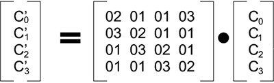
The new column is computed as follows:
C'0 = 02 * C0 + 01 * C1 + 01 * C2 + 03 * C3
C'1 = 03 * C0 + 02 * C1 + 01 * C2 + 01 * C3
C'2 = 01 * C0 + 03 * C1 + 02 * C2 + 01 * C3
C'3 = 01 * C0 + 01 * C1 + 03 * C2 + 02 * C3
Remember that we are not using normal arithmetic—we are using finite field arithmetic, which has special rules and both the multiplications and additions can be implemented using XOR.
After the MixColumns operation, the XorRoundKey is very simple indeed and hardly needs its own name. This operation simply takes the existing state array, XORs the value of the appropriate round key, and replaces the state array with the result. It is done once before the rounds start and then once per round, using each of the round keys in turn.
As you might expect, decryption involves reversing all the steps taken in encryption using inverse functions:
InvSubBytes
InvShiftRows
InvMixColumns
XorRoundKey doesn't need an inverse function because XORing twice takes you back to the original value. InvSubBytes works the same way as SubBytes but uses a different table that returns the original value. InvShiftRows involves rotating left instead of right and InvMixColumns uses a different constant matrix to multiply the columns.
The order of operation in decryption is:
Perform initial decryption round:
XorRoundKey
InvShiftRows
InvSubBytes
Perform nine full decryption rounds:
XorRoundKey
InvMixColumns
InvShiftRows
InvSubBytes
Perform final XorRoundKey
The same round keys are used in the same order.
Now we have seen all the steps needed to take a 128-bit block of data and transform it into ciphertext. We also looked at the reverse process for decryption. The process of encryption can be summarized as shown in Figure A.3. The mathematics behind the algorithm is rather hard to understand for nonmathematicians and we have focused on how rather than why in this book. If you are interested in such matters, it is probably worth reading the theoretical papers of looking at the book that specialize in cryptography. What is interesting, however, is the way in which all the operations are based on byte values and operations that are simple to implement in digital logic gates. AES achieves the goal of being both secure and practical for real systems.
