© Nicolas Modrzyk 2020
N. ModrzykReal-Time IoT Imaging with Deep Neural Networkshttps://doi.org/10.1007/978-1-4842-5722-7_2

2. Object Detection in Video Streams

Nicolas Modrzyk1 
(1)
Tokyo, Tokyo, Japan
 

Most of the available how-to guides for working with OpenCV in Java require you to have an insane amount of knowledge before getting started. The good news for you is that with what you have learned up to now with this book, you can get started with OpenCV in Java in seconds.

Going Sepia: OpenCV Java Primer

Choosing sepia is all to do with trying to make the image look romantic and idealistic. It’s sort of a soft version of propaganda.

—Martin Paar1

In this section, you will be introduced to some basic OpenCV concepts . You’ll learn how to add the files needed for working with OpenCV in Java, and you’ll work on a few simple OpenCV applications, like smoothing, blurring images, or indeed turning them into sepia images.

A Few Files to Make Things Easier…

Visual Studio Code is clever, but to understand the code related to the OpenCV library, it needs some instructions. Those instructions are included in a project’s metadata file, which specifies what library and what version to include to run the code.

A template for OpenCV/Java has been prepared for you, so to get started, you can simply clone the project template found here:
git clone [email protected]:hellonico/opencv-java-template.git
Or you can use the zip file, found here:
https://github.com/hellonico/opencv-java-template/archive/master.zip
This will give you the minimum set of files required, as shown here:
.
├── pom.xml
└── src
    ├── main
    │   └── java
    │       └── hello
    │           └── HelloCv.java
    └── test
        └── java
            └── hello
                └── AppTest.java
There are seven directories and three files. Since this setup can be autogenerated, let’s focus on the template content, listed here:
  • HelloCv.java, which contains the main Java code

  • AppTest.java, which contains the bare minimum Java test file

  • pom.xml, which is a project descriptor that Visual Studio Code can use to pull in external Java dependencies

You can open that top folder from the project template from within Visual Studio Code, which gives you a familiar view, as shown in Figure 2-1.
../images/490964_1_En_2_Chapter/490964_1_En_2_Fig1_HTML.jpg
Figure 2-1

Project layout

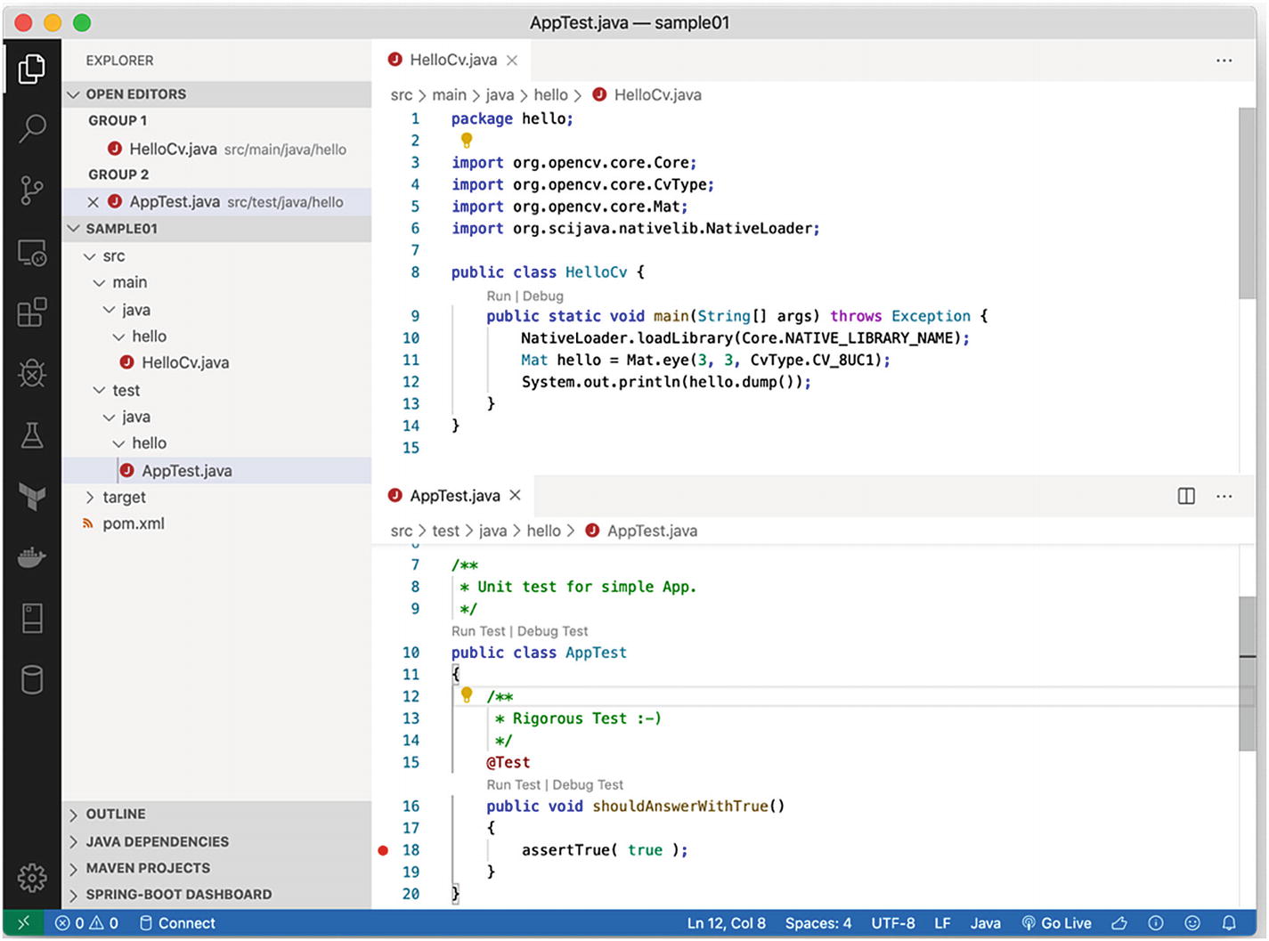
Figure 2-1 shows the two Java files, so you can see the content of each; in addition, the project layout has been expanded so all the files are listed on the left.

This view should look familiar to you from the previous chapter, and you can immediately try running the HelloCv.java code using the Run or Debug link at the top of the main function.

The output in the terminal should look like the following code, which is an OpenCV Mat object. To put it simply, it’s a matrix of size 3×3, with 1 on the top-left, bottom-right diagonal.
[  1,   0,   0;
   0,   1,   0;
   0,   0,   1]
Listing 2-1 probably looks familiar to users of OpenCV.
package hello;
import org.opencv.core.Core;
import org.opencv.core.CvType;
import org.opencv.core.Mat;
import org.scijava.nativelib.NativeLoader;
public class HelloCv {
    public static void main(String[] args) throws Exception {
        NativeLoader.loadLibrary(Core.NATIVE_LIBRARY_NAME);
        Mat hello = Mat.eye(3, 3, CvType.CV_8UC1);
        System.out.println(hello.dump());
    }
}
Listing 2-1

First OpenCV Mat

Let’s go through the code line by line to understand what is happening behind the scenes.

First, we use the NativeLoader class to load a native library, as shown here:
NativeLoader.loadLibrary(Core.NATIVE_LIBRARY_NAME);

This step is required because OpenCV is not a Java library; it is a binary compiled especially for your environment.

Usually in Java, you load a native library with System.loadLibrary , but that requires these two things:
  • You have a library compiled for your machine.

  • The library is placed somewhere where the Java runtime on your computer can find it.

In this book, we will rely on some packaging magic, where the library is downloaded and loaded automatically for you and where, along the way, the library is placed in a location that NativeLoader handles for you. So, there’s nothing to do here except to add that one-liner to the start of each of your OpenCV programs; it’s best to put it at the top of the main function.

Now, let’s move on to the second line of the program, as shown here:
Mat hello = Mat.eye(3, 3, CvType.CV_8UC1);

That second line creates a Mat object. A Mat object is, as explained a few seconds ago, a matrix. All image manipulation, all video handling, and all the networking are done using that Mat object. It wouldn’t be too much of a stretch to say that the main thing OpenCV is programmatically doing is proposing a great programming interface to work with optimized matrices, in other words, this Mat object.

In Visual Studio Code, you can already access operations directly using the autocompletion feature, as shown in Figure 2-2.
../images/490964_1_En_2_Chapter/490964_1_En_2_Fig2_HTML.jpg
Figure 2-2

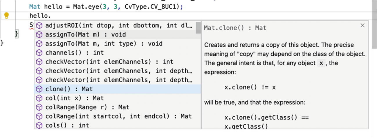
Inline documentation for the OpenCV Mat object

Within the one-liner, you create a 3×3 matrix, and the internal type of each element in the matrix is of type CV_8UC1. You can think of 8U as 8 bits unsigned, and you can think of C1 as channel 1, which basically means one integer per cell of the matrix.

The naming scheme for types is as follows:
 CV_<bit-depth>{U|S|F}C<number_of_channels>
Understanding the types used in Mat is important, so be sure to review the most common types shown in Table 2-1.
Table 2-1

OpenCV Types for OpenCV Mat Object

Name

Type

Bytes

Signed

Range

CV_8U

Integer

1

No

0 to 255

CV_8S

Integer

1

Yes

−128 to 127

CV_16S

Integer

2

Yes

−32768 to 32767

CV_16U

Integer

2

No

0 to 65535

CV_32S

Integer

4

Yes

−2147483648 to 2147483647

CV_16F

Float

2

Yes

−6.10 × 10⁻⁵ to 6.55 × 10⁴

CV_32F

Float

4

Yes

−1.17 × 10-38 to 3.40 × 1038

The number of channels in a Mat is also important because each pixel in an image can be described by a combination of multiple values. For example, in RGB (the most common channel combination in images), there are three integer values between 0 and 256 per pixel. One value is for red, one is for green, and one is for blue.

See for yourself in Listing 2-2, where we show a 50×50 blue Mat.
public class HelloCv2 {
    public static void main(String[] args) throws Exception {
        NativeLoader.loadLibrary(Core.NATIVE_LIBRARY_NAME);
        Mat hello = Mat.eye(50, 50, CvType.CV_8UC3);
        hello.setTo(new Scalar(190, 119, 0));
        HighGui.imshow("rgb", hello);
        HighGui.waitKey();
        System.exit(0);
    }
}
Listing 2-2

Some Blue…

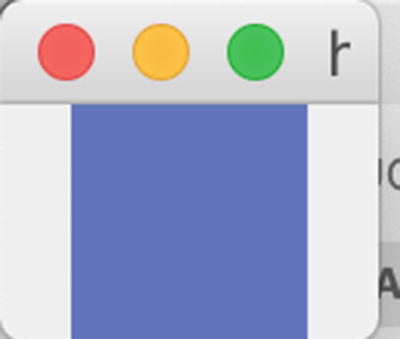
Executing the previous code will give you this 50×50 Mat, where each pixel is made of three channels, meaning three values, but note that in OpenCV, RGB values are reversed by design (why, oh, why?), so it is actually BGR. The value for blue comes first in the code.
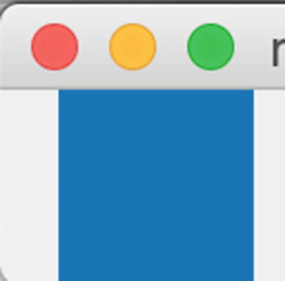
So, before the value of all the pixels, set using the function setTo, is B:190, G:119, Red:0, which gives the nice ocean sea blue shown in Figure 2-3.
../images/490964_1_En_2_Chapter/490964_1_En_2_Fig3_HTML.jpg
Figure 2-3

Sea blue

Operations on Mat objects are usually done using the org.opencv.core.Core class. For example, adding two Mat objects is done using the Core.add function, two input objects, two Mat objects, and a receiver for the result of the addition, which is another Mat.

To understand this, we can use a 1×1 Mat object. You can see that when adding two Mat objects together, you get a resulting Mat where each cell value is the result of the addition of the same location in the first Mat and the second Mat. Finally, the result is stored in dest Mat, as shown in Listing 2-3.
Mat hello = Mat.eye(1, 1, CvType.CV_8UC3);
hello.setTo(new Scalar(190, 119, 0));
Mat hello2 = Mat.eye(1, 1, CvType.CV_8UC3);
hello2.setTo(new Scalar(0, 0, 100));
Mat dest = new Mat();
Core.add(hello, hello2, dest);
System.out.println(dest.dump());
Listing 2-3

Adding Two Mat Objects Together

The result is shown in the following 1×1 dest Mat. Don’t get confused; this is only one pixel with three values, one per channel.
[190, 119, 100]

Now, we’ll let you practice a little bit and perform the same operation on a 50×50 Mat and show the result in a window again with HighGui.

The result should look like Figure 2-4.
../images/490964_1_En_2_Chapter/490964_1_En_2_Fig4_HTML.jpg
Figure 2-4

Adding two colored Mats

OpenCV Primer 2: Loading, Resizing, and Adding Pictures

You’ve seen how to add super small Mat objects together, but let’s see how things work when adding two pictures , specifically, two big Mat objects, together.

My sister has a beautiful cat, named Marcel, and she very nicely agreed to provide a few pictures of Marcel to use for this book. Figure 2-5 shows Marcel taking a nap.
../images/490964_1_En_2_Chapter/490964_1_En_2_Fig5_HTML.jpg
Figure 2-5

Marcel at work

I’ve never seen Marcel at the beach, but I would like to have a shot of him near the ocean.

In OpenCV, we can achieve this by taking Marcel’s picture and adding it to a picture of the beach (Figure 2-6).
../images/490964_1_En_2_Chapter/490964_1_En_2_Fig6_HTML.jpg
Figure 2-6

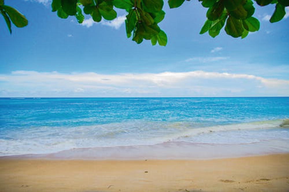
The beach where Marcel is heading to

Adding these two pictures together properly is going to take just a bit of work the first time, but it will be useful to understand how OpenCV works.

Simple Addition

Loading a picture is done using the imread function from the Imgcodec class. Calling imread with a path returns a Mat object, the same kind of object you have been working with so far. Adding the two Mats (the Marcel Mat and the beach Mat) is as simple as using the same Core.add function as used earlier, as shown in Listing 2-4.
Mat marcel = Imgcodecs.imread("marcel.jpg");
Mat beach = Imgcodecs.imread("beach.jpeg");
Mat dest = new Mat();
Core.add(marcel, beach, dest);
Listing 2-4

First Try at Adding Two Mats
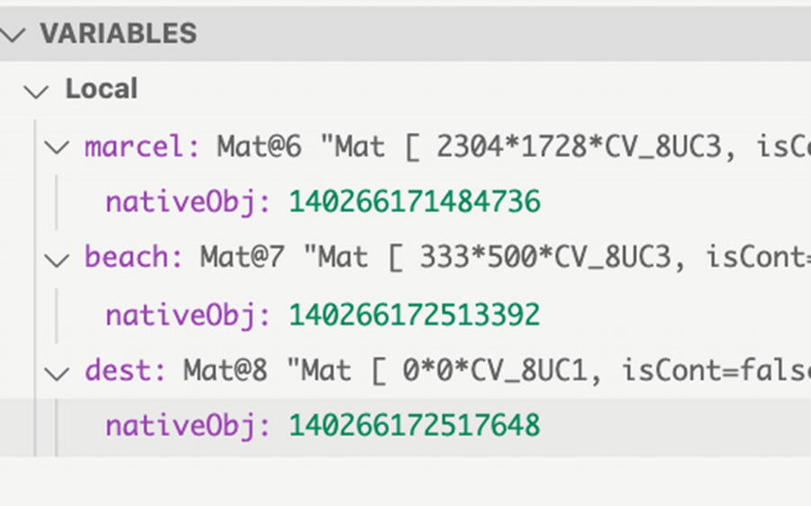
However, running the code for the first time returns an obscure error message, as shown here:
Exception in thread "main" CvException [org.opencv.core.CvException: cv::Exception: OpenCV(4.1.1) /Users/niko/origami-land/opencv-build/opencv/modules/core/src/arithm.cpp:663: error: (-209:Sizes of input arguments do not match) The operation is neither 'array op array' (where arrays have the same size and the same number of channels), nor 'array op scalar', nor 'scalar op array' in function 'arithm_op']
        at org.opencv.core.Core.add_2(Native Method)
        at org.opencv.core.Core.add(Core.java:1926)
        at hello.HelloCv4.simplyAdd(HelloCv4.java:16)
        at hello.HelloCv4.main(HelloCv4.java:41)
Don’t get scared; let’s quickly check with the debugger what is happening and add a breakpoint at the proper location; see the Mat objects on the Variables tab, as shown in Figure 2-7.
../images/490964_1_En_2_Chapter/490964_1_En_2_Fig7_HTML.jpg
Figure 2-7

Debugging Mats

Before adding a breakpoint, we can see that the Marcel Mat is indeed 2304×1728, while the beach Mat is smaller at 333×500, so we definitely need to resize the second Mat to match that of Marcel. If we do not perform this resizing step, OpenCV does not know how to compute the result of the add function and gives the error message shown earlier.

Our second try produces the code in Listing 2-5, where we use the resize function of class Imgproc to change the beach Mat to be the same size as the Marcel Mat.
Mat marcel = Imgcodecs.imread("marcel.jpg");
Mat beach = Imgcodecs.imread("beach.jpeg");
Mat dest = new Mat();
Imgproc.resize(beach, dest, marcel.size());
Core.add(marcel, dest, dest);
Imgcodecs.imwrite("marcelOnTheBeach.jpg", dest);
Listing 2-5

Resizing

Running this code, the output image looks similar to Figure 2-8.
../images/490964_1_En_2_Chapter/490964_1_En_2_Fig8_HTML.jpg
Figure 2-8

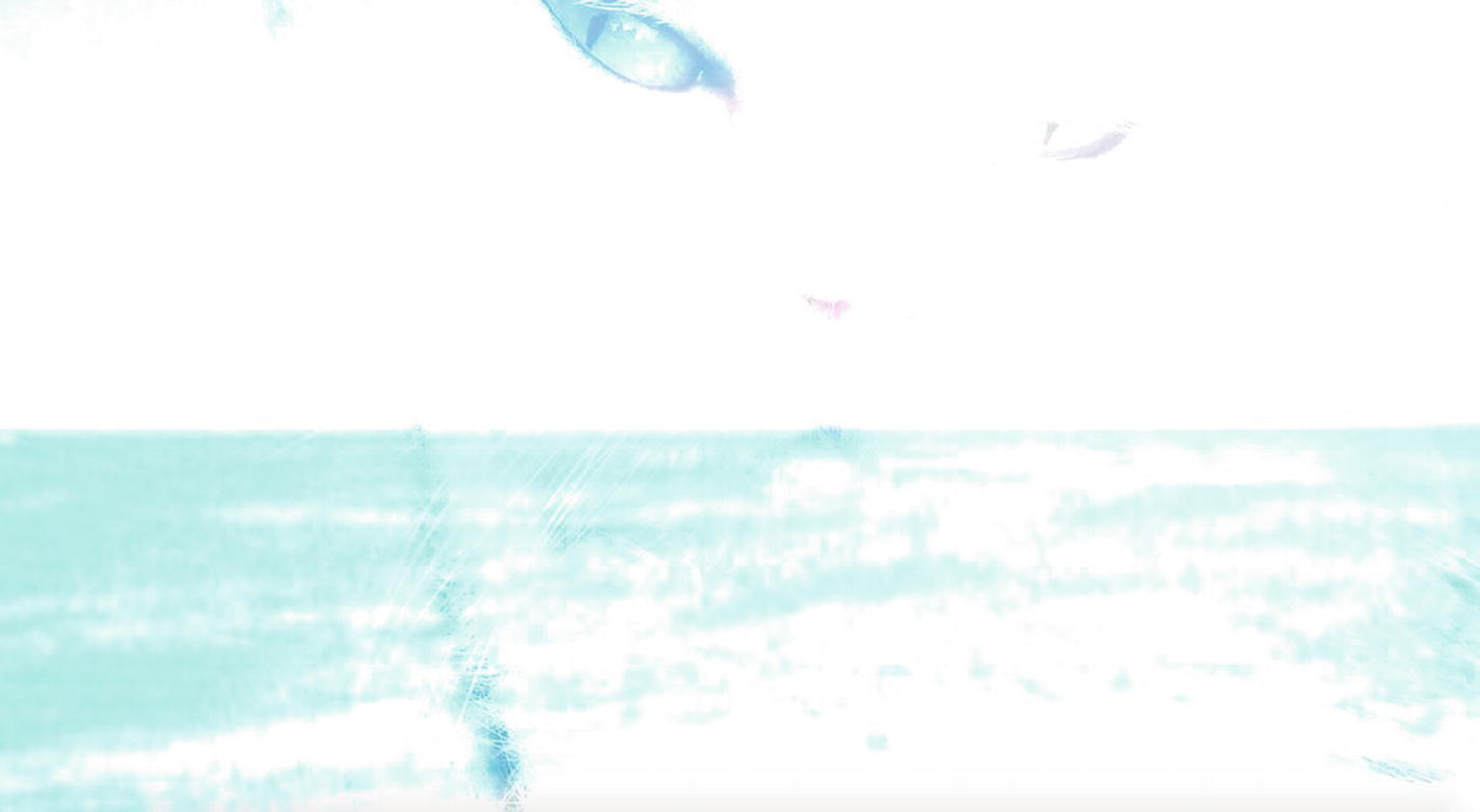
White, white, very white Marcel at the beach

Hmm. It’s certainly better because the program runs to the end without error, but something is not quite right. The output picture gives an impression of being over-exposed, and looks way too bright. And indeed, if you look, most of the output image pixels have maximum RGB values of 255,255,255, which is the RGB value for white.

We should do an addition in a way that keeps the feeling of each Mat but still not goes over the maximum 255,255,255 value.

Weighted Addition

Preserving meaningful values in Mat objects is certainly something that OpenCV can do. The Core class comes with a weighted version of the add function that is conveniently named addWeighted. What addWeighted does is multiply values of each Mat object, each by a different scaling factor. It’s even possible to adjust the result value with a parameter called gamma.

The function addWeighted takes no less than six parameters; let’s review them one by one.
  • The input image1

  • alpha, the factor to apply to image1’s pixel values

  • The input image2

  • beta, the factor to apply to image2’s pixel values

  • gamma, the value to add to the sum

  • The destination Mat

So, to compute each pixel of the result Mat object, addWeighted does the following:
image1 x alpha + image2 x beta + gamma = dest
Replacing Core.add with Core.addWeighted and using some meaningful parameter values, we now get the code shown in Listing 2-6.
Mat marcel = Imgcodecs.imread("marcel.jpg");
Mat beach = Imgcodecs.imread("beach.jpeg");
Mat dest = new Mat();
Imgproc.resize(beach, dest, marcel.size());
Core.addWeighted(marcel, 0.8, dest, 0.2, 0.5, dest);
Listing 2-6

Marcel Goes to the Beach

The output of the program execution gives something much more useful, as shown in Figure 2-9.
../images/490964_1_En_2_Chapter/490964_1_En_2_Fig9_HTML.jpg
Figure 2-9

addWeighted. Marcel can finally relax at the beach

Back to Sepia

At this stage, you know enough about Mat computation in OpenCV that we can go back to the sepia example presented a few pages earlier.

In the sepia sample, we were creating a kernel, another Mat object, to use with the Core.transform function .

Core.transform applies a transformation to the input image where
  • The number of channels of each pixel in the output equals the number of rows of the kernel.

  • The number of columns in the kernel must be equal to the number of channels of the input, or +1.

  • The output value of each pixel is a matrix transformation, and the matrix transformation of every element of the array src stores the results in dst, where dst[ I ] = m x src[ I ].

See Table 2-2 for examples of how this works.
Table 2-2

Core.transform Samples

Source

Kernel

Output

Computation

[2 3]

[5]

[10 15]

10 = 2 × 5

15 = 3 × 5

[2 3]

[5 1]

[11 16]

11 = 2 × 5 + 1

16 = 3 × 5 + 1

[2 3]

[5

10]

[(10, 20) (15, 30)]

(10 = 2 × 5

20 = 2 × 10)

(15 = 3 × 5

30 = 3 × 10)

[2]

[1 2

3 4]

[(4 10)]

4 = 2 × 1 + 2

10 = 3 × 2 + 4

[2 3]

[1 2

3 4]

[(4 10) (5 13)]

4 = 2 × 1 + 2

10 = 2 × 3 + 4

5 = 3 × 1 + 2

13 = 3 × 3 + 4

[2]

[1

2

3]

[(2 4 6)]

2 = 2 × 1

4 = 2 × 2

6 = 2 × 3

[2]

[1 2

3 4

5 6]

[(4 10 16)]

4 = 2 × 2 + 1

10 = 2 × 3 + 4

16 = 2 × 5 + 6

[(190 119 10)]

[0.5 0.2 0.3]

[122]

122 = 190 × 0.5 + 119 × 0.2 + 10 × 0.3

The OpenCV Core.transform function can be used in many situations and is also at the root of turning a color image into a sepia one.

Let’s see whether Marcel can be turned into sepia. We apply a straightforward transform with a 3×3 kernel, where each value is computed as was just explained.

The simplest and most famous sepia transform uses a kernel with the following values:
[     0.272 0.534 0.131
      0.349 0.686 0.168
      0.393 0.769 0.189]
So, for each resulting pixel, the value for blue is as follows:
0.272 x Source Blue + 0.534 x Source Green + 0.131 x Source Red
The target value for green is as follows:
0.349 x Source Blue + 0.686 x Source Green + 0.168 x Source Red
Finally, the value for red is as follows:
0.393 x Source Blue + 0.769 x Source Green + 0.189 x Source Red
.

As, you can see, the values for red are largely pinned down, with each multipliers around 0.1, and green has the most impact on the pixel values for the resulting Mat objects.

The input image of Marcel this time is shown in Figure 2-10.
../images/490964_1_En_2_Chapter/490964_1_En_2_Fig10_HTML.jpg
Figure 2-10

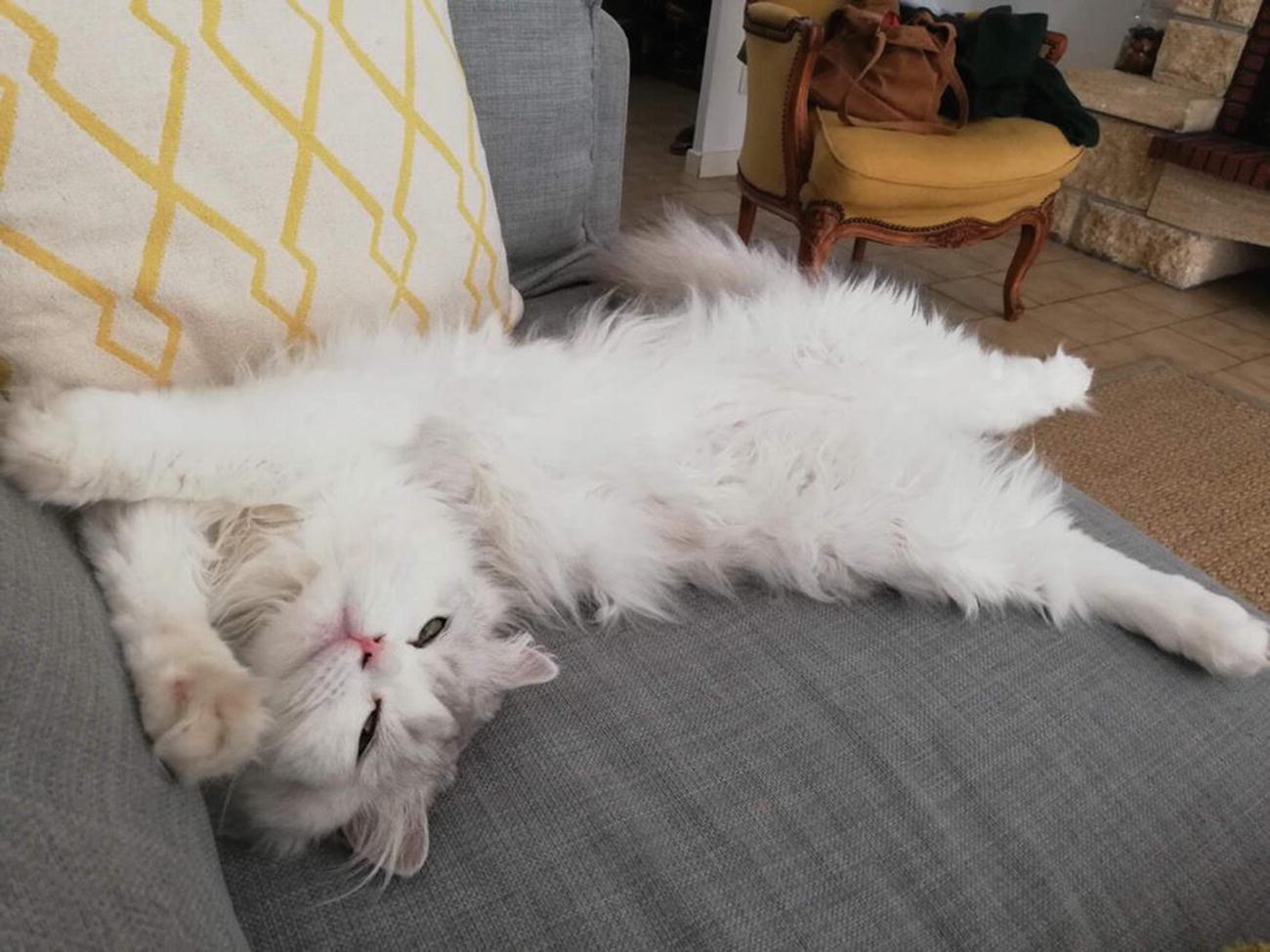
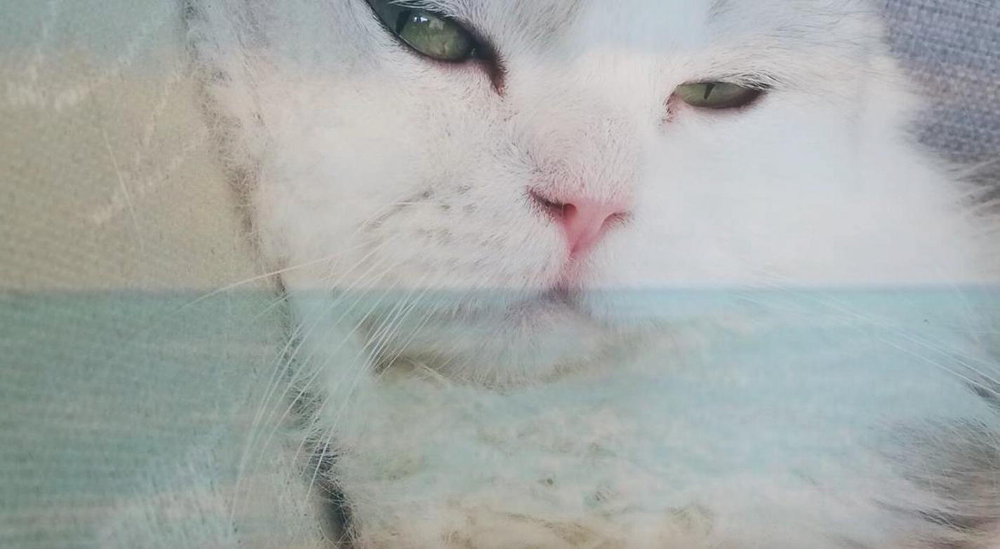
Marcel does not know he’s going to turn into sepia soon

To turn Marcel into sepia, first we read a picture using imread, and then we apply the sepia kernel, as shown in Listing 2-7.
Mat marcel = Imgcodecs.imread("marcel.jpg");
Mat sepiaKernel = new Mat(3, 3, CvType.CV_32F);
sepiaKernel.put(0, 0,
        // bgr -> blue
        0.272, 0.534, 0.131,
        // bgr -> green
        0.349, 0.686, 0.168,
        // bgr -> red
        0.393, 0.769, 0.189);
Mat destination = new Mat();
Core.transform(marcel, destination, sepiaKernel);
Imgcodecs.imwrite("sepia.jpg", destination);
Listing 2-7

Sepia Marcel

As you can see, the BGR output of each pixel is computed from the value of each channel of the same pixel in the input.

After we run the code, Visual Studio Code outputs the picture in a file named sepia.jpg, as in Figure 2-11.
../images/490964_1_En_2_Chapter/490964_1_En_2_Fig11_HTML.jpg
Figure 2-11

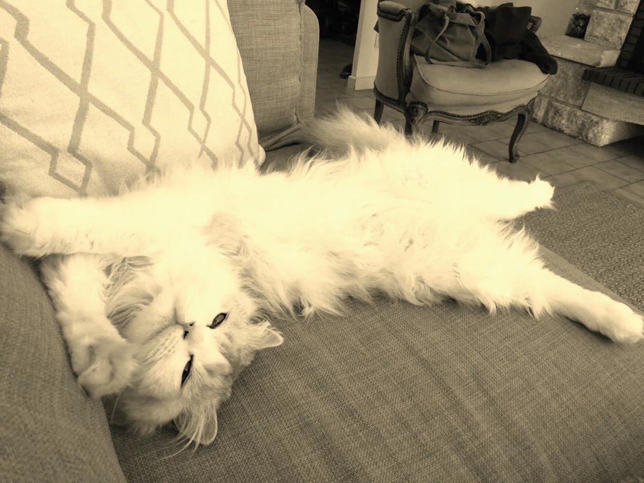
Marcel turned into sepia

That was a bit of yellowish sepia. What if we need more red? Go ahead and try it.

Increasing the red means increasing the values of the R channel, which is the third row of the kernel matrix.

Upping the value of kernel[3,3] from 0.189 to 0.589 gives more power to the red in the input to the red in the output. So, with the following kernel, Marcel turns into something redder, as shown in Figure 2-12:
// bgr -> blue
0.272, 0.534, 0.131,
// bgr -> green
0.349, 0.686, 0.168,
// bgr -> red
0.393, 0.769, 0.589
../images/490964_1_En_2_Chapter/490964_1_En_2_Fig12_HTML.jpg
Figure 2-12

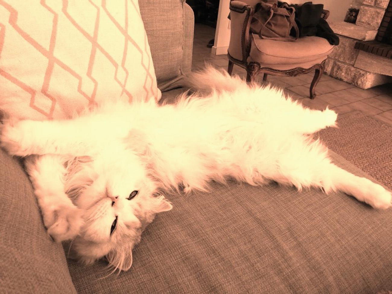
Red sepia version of Marcel

You can play around and try a few other values for the kernel so that the sepia turns greener or bluer…and of course try it with your own cat if you have one. But, can you beat the cuteness of Marcel?

Finding Marcel: Detecting Objects Primer

Let’s talk about how to detect objects using Marcel the cat.

Finding Cat Faces in Pictures Using a Classifier

Before processing speeds got faster and neural networks were making the front pages of all the IT magazines and books, OpenCV implemented a way to use classifiers to detect objects within pictures.

Classifiers are trained with only a few pictures, using a method that feeds the classifier with training pictures and the features you want the classifier to detect during the detection phase.

The three main types of classifiers in OpenCV, named depending on the type of features they are extracting from the input images during the training phase, are as follows:
  • Haar features

  • Hog features

  • Local binary pattern (LBP) features

The OpenCV documentation on cascade classifiers (https://docs.opencv.org/4.1.1/db/d28/tutorial_cascade_classifier.html) is full of extended details when you want to get some more background information. For now, the goal here is not to repeat this freely available documentation.

What Is a Feature?

Features are key points extracted from a set of digital pictures used for training, something that can be reused for matching on totally new digital inputs.

For example, an ORB classifier, nicely explained in “Object recognition with ORB and its Implementation on FPGA” (http://citeseerx.ist.psu.edu/viewdoc/download?doi=10.1.1.405.9932&rep=rep1&type=pdf) is a very fast binary descriptor based on BRIEF. The other famous feature-based algorithms are Scale Invariant Feature Transform (SIFT) and Speed Up Robust Features (SURF); all these are looking to match features for a set of known images (what we are looking for) on new inputs.

Listing 2-8 shows a super-brief example of how feature extraction is done. Here we are using an ORB detector to find the key points of a picture.
Mat src = Imgcodecs.imread("marcel2.jpg", Imgcodecs.IMREAD_GRAYSCALE);
ORB detector = ORB.create();
MatOfKeyPoint keypoints = new MatOfKeyPoint();
detector.detect(src, keypoints);
Mat target = src.clone();
target.setTo(new Scalar(255, 255, 255));
Features2d.drawKeypoints(target, keypoints, target);
Imgcodecs.imwrite("orb.png", target);
Listing 2-8

ORB Feature Extraction

Basically, the features are extracted into a set of points. We don’t do that usually, but drawing the key points here gives something like Figure 2-13.
../images/490964_1_En_2_Chapter/490964_1_En_2_Fig13_HTML.jpg
Figure 2-13

Extracting ORB features on Marcel

Cascade classifiers are called that because they internally have a set of different classifiers, each of them getting a deeper, more detailed chance of a match at a cost of speed. So, the first classifier will be very fast and get a positive or a negative, and if positive, it will pass the task on to the next classifier for some more advanced processing, and so on.
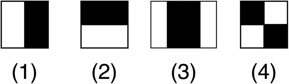
Haar-based classifiers, as proposed by Paul Viola and Michael Jones, are based on analyzing four main features, as shown in Figure 2-14.
../images/490964_1_En_2_Chapter/490964_1_En_2_Fig14_HTML.jpg
Figure 2-14

Haar feature types

Since the features are easily computed, the number of images required for training Haar-based object detection is quite low. Most importantly, up until recently, with low CPU speeds on embedded systems, those classifiers had the advantage of being very fast.

Where in the World Is Marcel?

So, enough talking and reading about research papers. In short, a Haar-based cascade classifier is good at finding features of faces, of humans or animals, and can even focus on eyes, noses, and smiles, as well as on features of a full body.

The classifiers can also be used to count the number of moving heads in video streams and find out whether anyone is stealing things from the fridge after bedtime.

OpenCV makes it a no-brainer to use a cascade classifier and get some instant gratification. The way to put cascade classifiers into action is as follows:
  1. 1.

    Load the classifier from an XML definition file containing values describing the features to look for.

     
  2. 2.

    Access a Mat object called detectMultiScale directly on the input Mat object, and a Mat object called MatOfRect, which is a specific OpenCV object designed to handle lists of rectangles nicely.

     
  3. 3.

    Once the previous call is finished, MatOfRect is filled with a number of rectangles, each of them describing a zone of the input image, where a positive has been found.

     
  4. 4.

    Do some artsy drawing on the original picture to highlight what was found by the classifier.

     
  5. 5.

    Save the output.

     
The Java code for this is actually rather simple and just barely longer than the equivalent Python code. See Listing 2-9.
String classifier
    = "haarcascade_frontalcatface.xml";
CascadeClassifier cascadeFaceClassifier
    = new CascadeClassifier(classifier);
Mat cat = Imgcodecs.imread("marcel.jpg");
MatOfRect faces = new MatOfRect();
cascadeFaceClassifier.detectMultiScale(cat, faces);
for (Rect rect : faces.toArray()) {
     Imgproc.putText(
       cat,
       "Chat",
      new Point(rect.x, rect.y - 5),
      Imgproc.FONT_HERSHEY_PLAIN, 10,
      new Scalar(255, 0, 0), 5);
     Imgproc.rectangle(
       cat,
       new Point(rect.x, rect.y),
       new Point(rect.x + rect.width, rect.y + rect.height),
      new Scalar(255, 0, 0),
      5);
}
Imgcodecs.imwrite("marcel_blunt_haar.jpg", cat);
Listing 2-9

Calling a Cascade Classifier on an Image
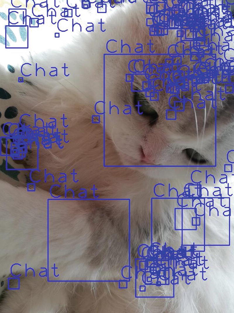
After running the code in Listing 2-9, you will realize quickly what the problem is with the slightly naïve approach. The classifier is finding a lot of extra positives, as shown in Figure 2-15.
../images/490964_1_En_2_Chapter/490964_1_En_2_Fig15_HTML.jpg
Figure 2-15

Too many Marcels…

There are two techniques to reduce the number of detected objects.
  • Filter the rectangles based on their sizes in the loop on rectangles. While this is often used thanks to its simplicity, this adds a chance to focus on false positives.

  • Pass in extra parameters to detectMultiScale, specifying, among other things, a certain number of required neighbors to get a positive or indeed a minimum size for the returned rectangles.

The full version has all the parameters shown in Table 2-3.
Table 2-3

detectMultiScale Parameters

Parameter

Description

image

Matrix of the type CV_8U containing an image where objects are detected.

objects

Vector of rectangles where each rectangle contains the detected object; the rectangles may be partially outside the original image.

scaleFactor

Parameter specifying how much the image size is reduced at each image scale.

minNeighbors

Parameter specifying how many neighbors each potential candidate rectangle should have to be retained.

flags

Not used for a new cascade.

minSize

Minimum possible object size. Objects smaller than this value are ignored.

maxSize

Maximum possible object size. Objects larger than this value are ignored if the maxSize == minSize model is evaluated on a single scale.

Based on the information from Table 2-3, let’s apply some sensible parameters to detectMutiScale, as shown here:
  • scalefactor=2

  • minNeighbors=3

  • flags=-1 (ignored)

  • size=300x300

Building on the code in Listing 2-9, let’s replace the line containing detectMultiScale with this updated one:
cascadeFaceClassifier.detectMultiScale(cat, faces, 2, 3, -1, new Size(300, 300));
Applying the new parameters, and (why not?) running a debug session on the new code, gives you the layout shown in Figure 2-16.
../images/490964_1_En_2_Chapter/490964_1_En_2_Fig16_HTML.jpg
Figure 2-16

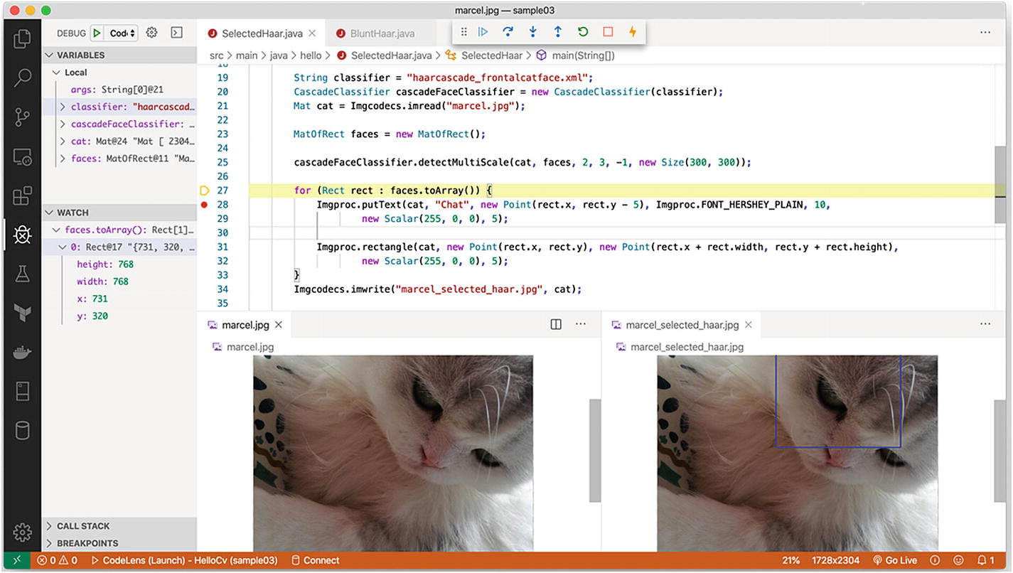
Debugging session while looking for Marcel

The output is already included in the layout, but you will notice the found rectangles are now limited to only one rectangle, and the output gives only one picture (and, yes, there can be only one Marcel).

Finding Cat Faces in Pictures Using the Yolo Neural Network

We have not really seen how to train cascade classifiers to recognize things we want them to recognize (because it’s beyond the scope of this book). The thing is, most classifiers have a tendency to recognize some things better than others, for example, people more than cars, turtles, or signs.

Detection systems based on those classifiers apply the model to an image at multiple locations and scales. High-scoring regions of the image are considered detections.

The neural network Yolo uses a totally different approach. It applies a neural network to the full image. This network divides the image into regions and predicts bounding boxes and probabilities for each region. These bounding boxes are weighted by the predicted probabilities.

Yolo has proven fast in real-time object detection and is going to be our neural network of choice to run in real time on the Raspberry Pi in Chapter 3.

Later, you will see how to train a custom Yolo-based model to recognize new objects that you are looking for, but to bring this chapter to a nice and exciting end, let’s quickly run one of the provided default Yolo networks, trained on the COCO image set, that can detect a large set of 80 objects, cats, bicycle, cars, etc., among other objects.

As for us, let’s see whether Marcel is up to the task of being detected as a cat even through the eyes of a modern neural network.

The final sample introduces a few more OpenCV concepts around deep neural networks and is a great closure for this chapter.

You probably know already what a neural network is; it is modeled on how the connections in the brain work, simulating threshold-based neurons triggered by incoming electrical signals. If my highly neuron-dense brain were a drawing, it would look something like Figure 2-17.
../images/490964_1_En_2_Chapter/490964_1_En_2_Fig17_HTML.jpg
Figure 2-17

My brain

I actually do hope reality is slightly different and my brain is way more colorful.

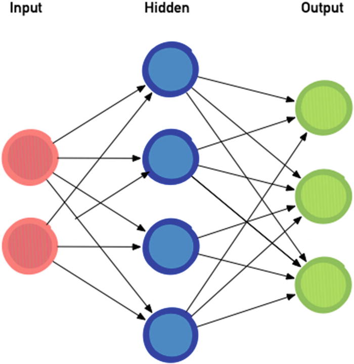
What you see in Figure 2-17 at first sight is the configuration of the network. Figure 2-17 shows only one hidden layer in between the input and output layers, but standard deep neural networks have around 60 to 100 hidden layers and of course way more dots for inputs and outputs.

In many cases, the network maps the image, with a hard-coded size specific to that network, from one pixel to one dot. The output is actually slightly more complicated, containing among other things probabilities and names, or at least an index of names in a list.

During the training phase, each of the arrows in the diagram, or each neuron connection in the network, is slowly getting a weight, which is something that impacts the value of the next neuron, which is a circle, in the next hidden or output layer.

When running the code sample, we will need both a config file for the graphic representation of the network, with the number of hidden layers and output layers, and a file for the weights, which includes a number for each connection between the circles.

Let’s move from theory to practice now with some Java coding. We want to give some file as the input to this Yolo-based network and recognize, you guessed it, our favorite cat.

The Yolo example is split into several steps, listed here:
  1. 1.

    Load the network as an OpenCV object using two files. As you have seen, this needs both a weight file and a config file.

     
  2. 2.

    In the loaded network, find out the unconnected layers, meaning the layers that do not have an output. Those will be output layers themselves. After running the network, we are interested in the values contained in those layers.

     
  3. 3.

    Convert the image we would like to detect objects from to a blob, something that the network can understand. This is done using the OpenCV function blobFromImage, which has many parameters but is quite easy to grasp.

     
  4. 4.

    Feed this beautiful blob into the loaded network, and ask OpenCV to run the network using the function forward. We also tell it the nodes we are interested in retrieving values from, which are the output layers we computed before.

     
  5. 5.
    Each output returned by the Yolo model is a set of the following:
    • Four values for the location (basically four values to describe the rectangle)

    • Values representing the confidence for each possible object that our network can recognize, in our case, 80

     
  6. 6.

    We move to a postprocess step where we extract and construct sets of boxes and confidences from the outputs returned by the network.

     
  7. 7.

    Yolo has a tendency to send many boxes for the same results; we use another OpenCV function, Dnn.NMSBoxes, that removes overlapping by keeping the box with the highest confidence score. This is called nonmaximum suppression (NMS).

     
  8. 8.

    We display all this on the picture using annotated rectangles and text, as is the case for many object detection samples.

     
See Listing 2-10 for the full code. Java, being verbose, results in quite a few lines, but this is not something you should be afraid of anymore. Right?
    static final String OUTFOLDER = "out/";
    static final Scalar BLACK = new Scalar(0, 0, 0);
    static {
        new File(OUTFOLDER).mkdirs();
    }
public static void main(String[] args) throws Exception {
    NativeLoader.loadLibrary(Core.NATIVE_LIBRARY_NAME);
    runDarknet(new String[] { "marcel.jpg", "marcel2.jpg", "chats.jpg", });
}
private static void runDarknet(String[] sourceImageFile) throws IOException {
    // read the labels
    List<String> labels = Files.readAllLines(Paths.get("yolov3/coco.names"));
    // load the network from the config and weights files
    Net net = Dnn.readNetFromDarknet("yolov3/yolov3.cfg", "yolov3/yolov3.weights");
    // look up for the output layers
    // this is network configuration dependent
    List<String> layersNames = net.getLayerNames();
    List<String> outLayers = net.getUnconnectedOutLayers().toList().stream().map(i -> i - 1).map(layersNames::get)
            .collect(Collectors.toList());
    // run the inference for each input
    for (String image : sourceImageFile) {
        runInference(net, outLayers, labels, image);
    }
}
private static void runInference(Net net, List<String> layers, List<String> labels, String filename) {
    final Size BLOB_SIZE = new Size(416, 416);
    final double IN_SCALE_FACTOR = 0.00392157;
    final int MAX_RESULTS = 20;
    // load the image, convert it to a blob, and
    // then feed it to the network
    Mat frame =
       Imgcodecs.imread(filename, Imgcodecs.IMREAD_COLOR);
    Mat blob = Dnn.blobFromImage(frame, IN_SCALE_FACTOR, BLOB_SIZE, new Scalar(0, 0, 0), false);
    net.setInput(blob);
    // glue code to receive the output of running the
    // network
    List<Mat> outputs = layers.stream().map(s -> {
        return new Mat();
    }).collect(Collectors.toList());
    // run the inference
    net.forward(outputs, layers);
    List<Integer> labelIDs = new ArrayList<>();
    List<Float> probabilities = new ArrayList<>();
    List<String> locations = new ArrayList<>();
    postprocess(filename, frame, labels, outputs, labelIDs, probabilities, locations, MAX_RESULTS);
}
private static void postprocess(String filename, Mat frame, List<String> labels, List<Mat> outs,
        List<Integer> classIds, List<Float> confidences, List<String> locations, int nResults) {
    List<Rect> tmpLocations = new ArrayList<>();
    List<Integer> tmpClasses = new ArrayList<>();
    List<Float> tmpConfidences = new ArrayList<>();
    int w = frame.width();
    int h = frame.height();
    for (Mat out : outs) {
        final float[] data = new float[(int) out.total()];
        out.get(0, 0, data);
        int k = 0;
        for (int j = 0; j < out.height(); j++) {
            // Each row of data has 4 values for location,
            // followed by N confidence values
            // which correspond to the labels
            Mat scores = out.row(j).colRange(5, out.width());
            // Get the value and location of the maximum score
            Core.MinMaxLocResult result =
                   Core.minMaxLoc(scores);
            if (result.maxVal > 0) {
                float center_x = data[k + 0] * w;
                float center_y = data[k + 1] * h;
                float width = data[k + 2] * w;
                float height = data[k + 3] * h;
                float left = center_x - width / 2;
                float top = center_y - height / 2;
                tmpClasses.add((int) result.maxLoc.x);
                tmpConfidences.add((float) result.maxVal);
                tmpLocations.add(
                  new Rect(
                         (int) left,
                   (int) top,
                         (int) width,
                         (int) height));
            }
            k += out.width();
        }
    }
    annotateFrame(frame, labels, classIds, confidences, nResults, tmpLocations, tmpClasses, tmpConfidences);
    Imgcodecs.imwrite(OUTFOLDER + new File(filename).getName(), frame);
}
private static void annotateFrame(Mat frame, List<String> labels, List<Integer> classIds, List<Float> confidences,
        int nResults, List<Rect> tmpLocations, List<Integer> tmpClasses, List<Float> tmpConfidences) {
    // Perform non maximum suppression to eliminate
    // redundant overlapping boxes with
    // lower confidences and sort by confidence
    // many overlapping results coming from yolo
    // so have to use it
    MatOfRect locMat = new MatOfRect();
    locMat.fromList(tmpLocations);
    MatOfFloat confidenceMat = new MatOfFloat();
    confidenceMat.fromList(tmpConfidences);
    MatOfInt indexMat = new MatOfInt();
    Dnn.NMSBoxes(locMat, confidenceMat, 0.1f, 0.1f, indexMat);
    // at this stage we only have the non-overlapping boxes,
    // with the highest confidence scores
    // so we draw them on the pictures.
    for (int i = 0; i < indexMat.total() && i < nResults; ++i) {
        int idx = (int) indexMat.get(i, 0)[0];
        classIds.add(tmpClasses.get(idx));
        confidences.add(tmpConfidences.get(idx));
        Rect box = tmpLocations.get(idx);
        String label = String.format("%s [%.0f%%]", labels.get(classIds.get(i)), 100 * tmpConfidences.get(idx));
        Imgproc.rectangle(frame, box, BLACK, 2);
        Imgproc.putText(frame, label, new Point(box.x, box.y), Imgproc.FONT_HERSHEY_PLAIN, 5.0, BLACK, 3);
    }
}
Listing 2-10

Running Yolo on Images

Running the example on images of Marcel actually brings really high confidence scores that are close to a perfect location, as shown in Figure 2-18.
../images/490964_1_En_2_Chapter/490964_1_En_2_Fig18_HTML.jpg
Figure 2-18

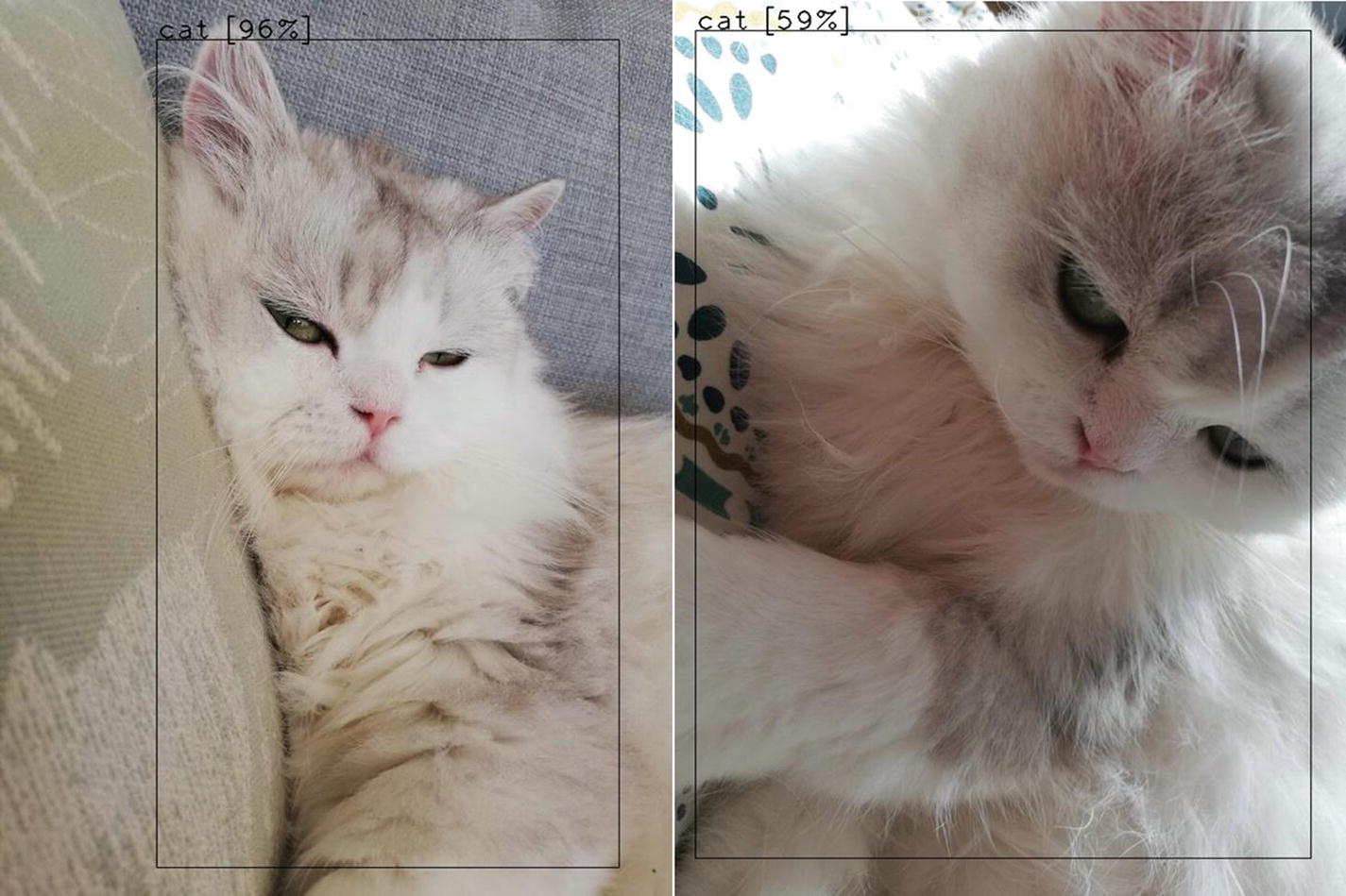
Yolo based detection confirms Marcel is a cute cat
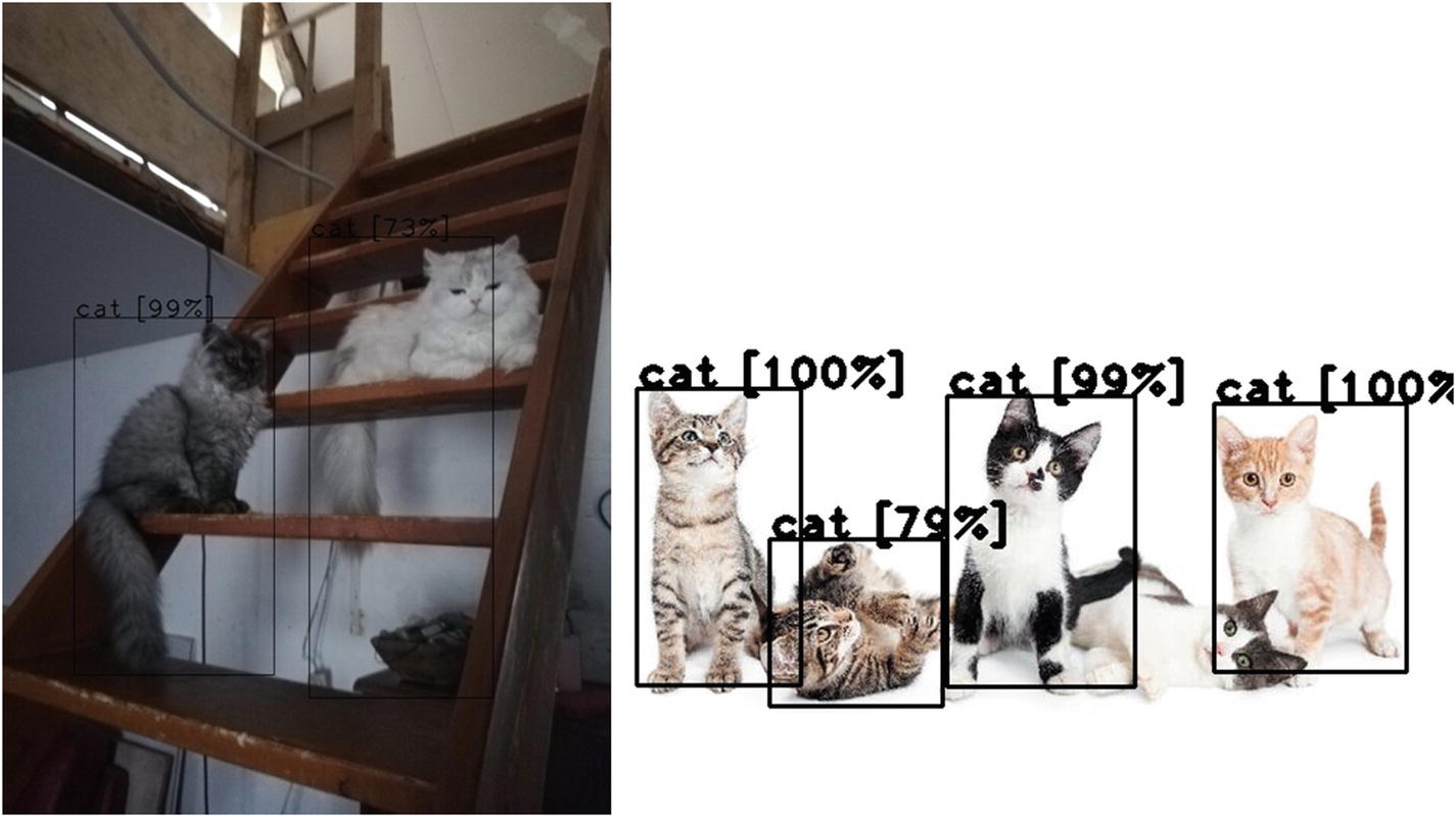
Running the inference on many cats also gives great results, but on the second run we are missing one of the cats because of its close position to another detected cat and because of our introduction of the postprocessing step, which removes overlapping matching boxes. See Figure 2-19.
../images/490964_1_En_2_Chapter/490964_1_En_2_Fig19_HTML.jpg
Figure 2-19

Many cats

An exercise for you at this point is to change the parameters of the Dnn.NMSBoxes function call to see whether you can get the two boxes to show at the same time.

The problem with static images is that it is difficult to get the extra context that we have in real life. This is a shortcoming that goes away when dealing with sets of input images coming from a live video stream.

So, with Chapter 2 wrapped up, you can now do object detection on pictures. Chapter 3 will take it from here and use the Raspberry Pi to teach you about on-device detection.

..................Content has been hidden....................

You can't read the all page of ebook, please click here login for view all page.
Reset
18.116.90.246