In this chapter, you’ll learn how to analyze video streams using concepts taken from functional programming. Specifically, you’ll use the Filter interface and combine it with a Pipeline object and then apply them to the video stream.
We will start with an overview of filters. Then we’ll look at different basic, fun filters, and we’ll gradually move on to object detection using different vision techniques. Finally, we’ll talk about neural networks.
Overview of Applying Filters
Read, Turn to Gray, Canny Resize, and Save
This is a Java book, though, so let’s see how we can apply the same concepts in Java.
Here we introduce the concept of a pipeline of filters, where each filter performs one operation on the Mat object.
Turning a Mat object to gray
Applying a Canny effect
Looking for edges
Pencil sketching
Instagram filters, like sepia or vintage
Doing background subtraction
Detecting cat or people faces using Haar objection detection or color detection
Running a neural network and identifying objects
The Filter interface, which consists of only one function, apply(Mat in), and returns a Mat object, just like in functional programming.
The Pipeline class, itself a Filter, that takes a list of classes or already instantiated filters. When apply is called, it applies the classes one by one.
The Filter Interface
Many Filters
Note here the usage of the deprecated version of the newInstance function directly in the class. This may not be calling the constructor you really want, but it works well enough for the examples in this book.
So far, Filter and Pipeline haven’t done a lot, of course, so let’s review some basic examples in the upcoming section.
Applying Basic Filters
In this section, we’ll look at several examples of basic filters.
Gray Filter
The most obvious use of a filter is to turn a Mat object from color to gray. In OpenCV, this is done using the function cvtColor from the Imgproc class.
Gray Filter on the Stream

Not only my hair, but the whole picture, is turning gray
Edge Preserving Filter
EdgePreservering Class Re-implemented as a Filter
Modified Main Function to Use Edge Preserving Filter

Edge Preserving filter
Canny
OpenCV’s Canny in a Filter
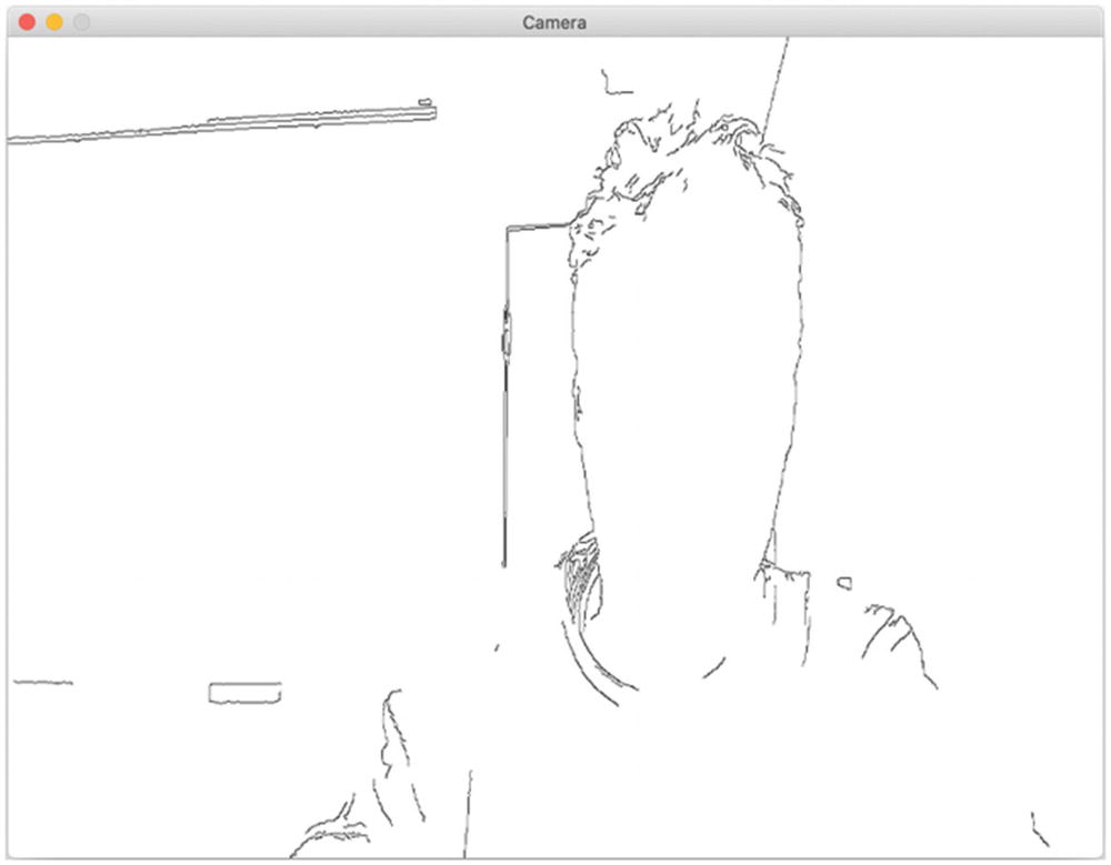
Canny filter on webcam stream
Debugging (Again)
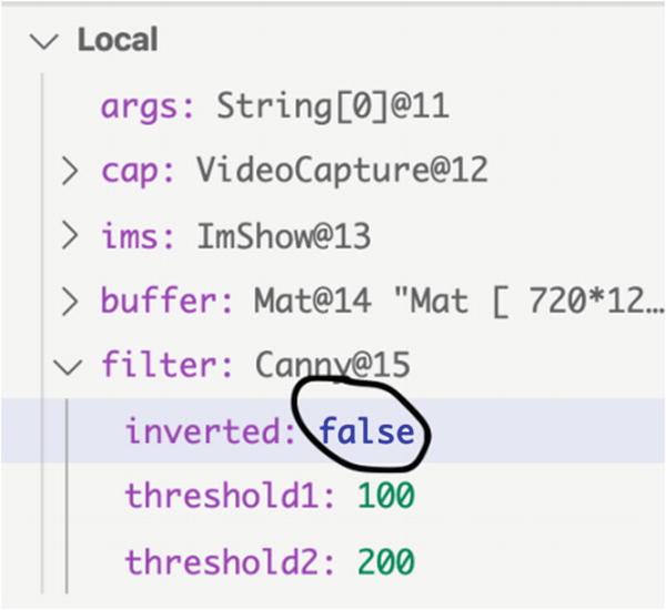
Updating the filter parameters in real time
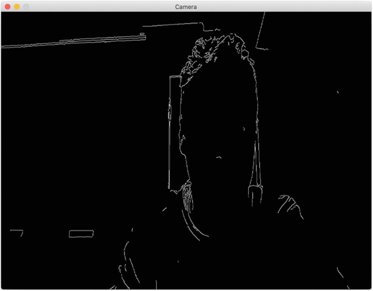
Noninverted Canny filter
When implementing your own filters, it’s a good idea to keep the most influential variables as fields of the class so you’re not flooded with values but still have access to the important ones.
Combining Filters
You probably realized in the previous sections that you will want to find out the performance of each filter.
Performance actually results from how many frames per seconds you can handle when reading from the video file or directly from the webcam device.
Display the frame rate directly on the image
Combine a Gray filter with the Framerate filter using the Pipeline class we defined earlier in this chapter
We already have the code for the Gray filter, so we’ll move directly to the code for displaying the frame rate per second (FPS).
I always thought I could access the value of the frame rate using OpenCV’s set of properties on VideoCapture. Unfortunately, we’re pretty much always stuck with a hard-coded value and not what is actually showing on the screen.
So, the implementation of FPS in Listing 4-8 is a small work-around that does some simple arithmetic based on how many frames have been displayed since the beginning of the filter’s life.
FPS Filter
Now let’s get back to combining the FPS showing on the stream with the Gray filter.

Combined Gray filter with FPS
Applying Instagram-like Filters
Enough serious work for now. Let’s take a short break and have a bit of fun with some Instagram-like filters.
Color Map
Color Map
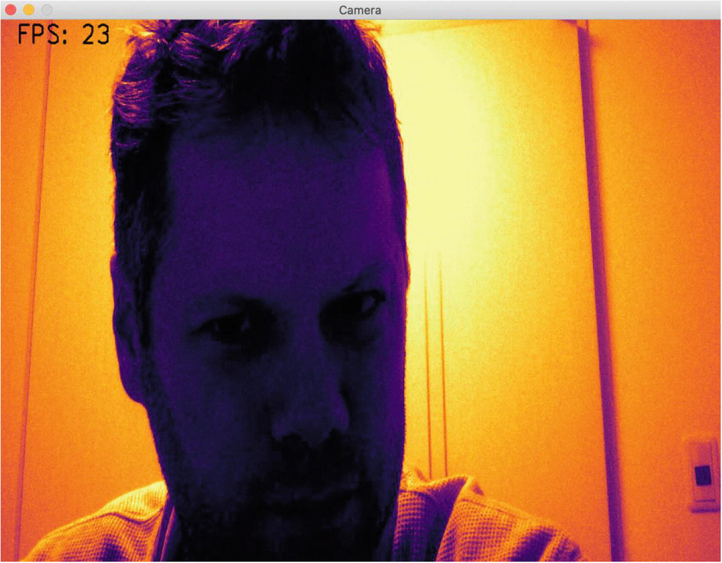
Inferno
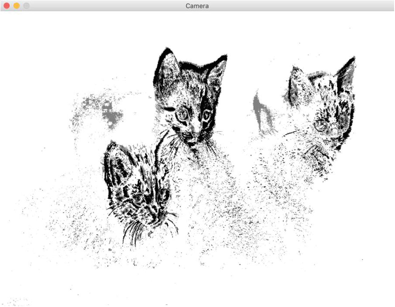
Thresh
Thresh is another fun filter made by applying the threshold function of Imgproc. It applies a fixed-level threshold to each array element of the Mat object.
The original purpose of the Thresh filter was to segment elements of a picture, such as to remove the noise of a picture by removing unwanted elements. It is not usually used for Instagram filtering, but it does look nice and can give you some creative ideas.
Applying Threshold
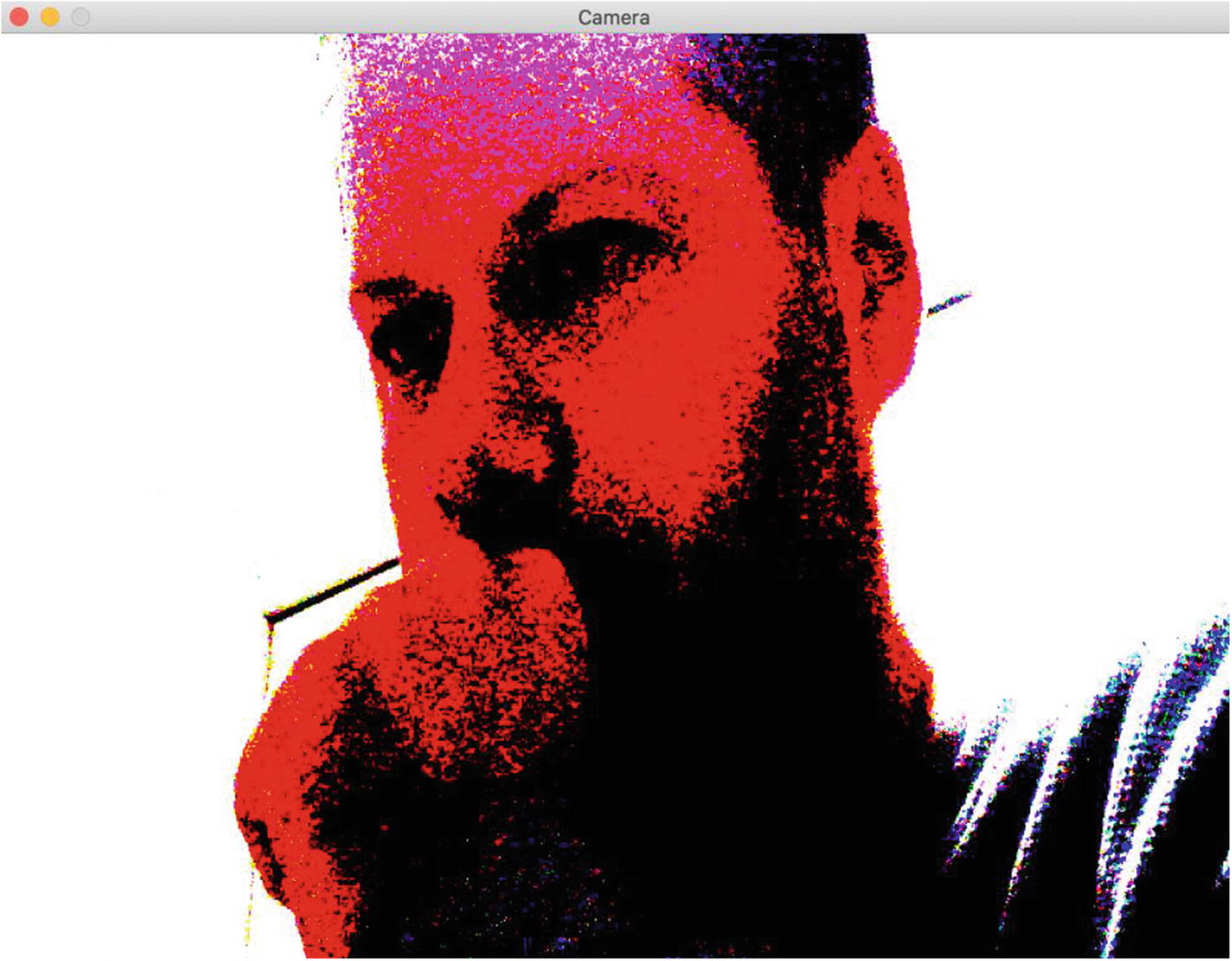
Applying Thresh for a burning effect
Sepia
Sepia
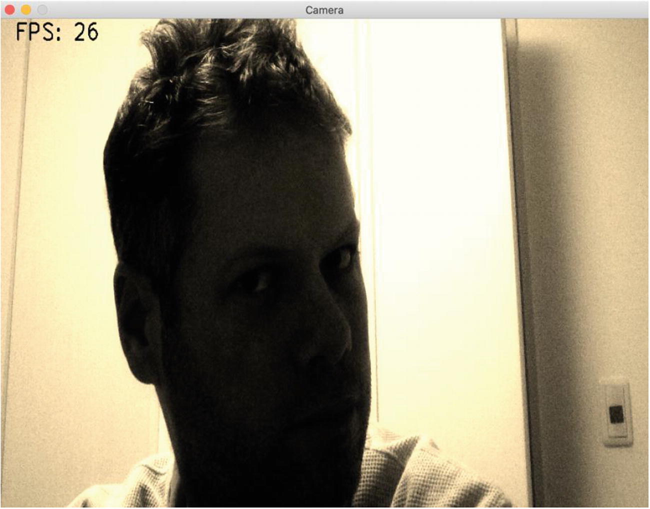
Sepia effect
Cartoon
Cartoon Filter
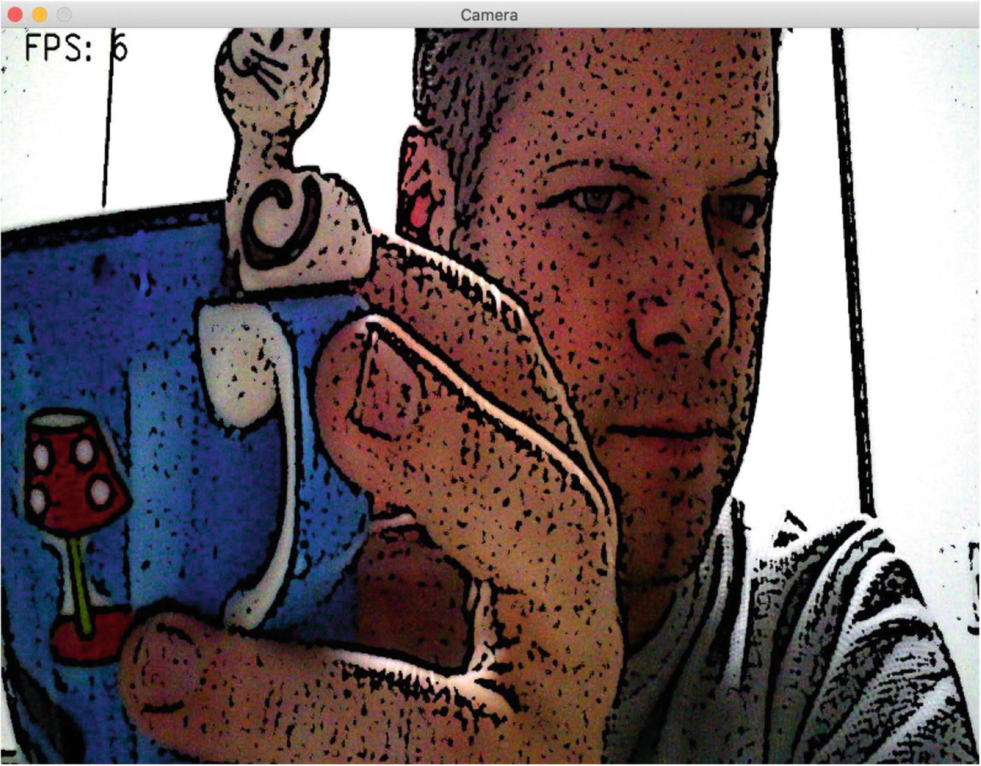
Cartoon effect
Pencil Effect
Pencil Effect
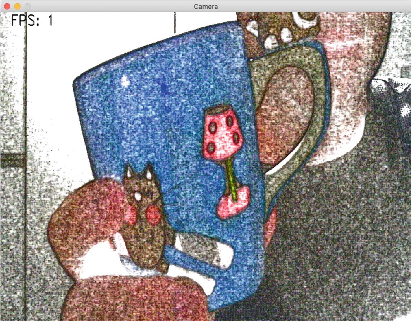
Pencil sketching
Woo-hoo. That was quite a few effects ready to use and apply for leisure. There are a few others available in the origami repositories, and you can of course contribute your own, but for now, let’s move on to serious object detection.
Performing Object Detection
Object detection is the concept of finding an object within a picture using different programming algorithms. It is a task that has long been done by human beings and that was quite hard for brain-less computers to do. But that has changed recently with advances in technology.
Using a simple contours-drawing filter
Detecting objects by colors
Using Haar classifiers
Using template matching
Using a neural network like Yolo
The examples go in somewhat progressive order of difficulty, so it’s best to try them in the order of this list.
Removing the Background
Removing the background is a technique you can use to remove unnecessary artifacts from a scene. The objects you are trying to find are probably not static and are likely to be moving across the set of pictures or video streams. To remove artefacts efficiently the algorithm needs to be able to differentiate two Mat objects and use some kind of short-term memory to differentiate moving things (in the foreground) from standard scene objects in the background.
Basically, you give more and more frames to the background subtractor, which can then detect what is moving in the foreground and what is not.
BackgroundSubtractor Class
Removing the background
Once you have this filter running, try switching to the KNN-based BackgroundSubtractor and see the difference in speed (looking at the frame rate) and the accuracy of the results.
Detecting by Contours
The second most basic OpenCV feature is to be able to find the contours in an image. The Contours filter uses the findContours function from the Imgproc class.
Turn the input Mat object to gray
Apply a Canny filter
Detecting Contours
with a Contours filter that just extracts contours. Try it!
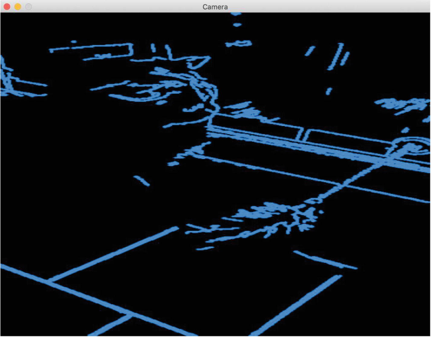
Using OpenCV’s detecting contours feature
Here’s an exercise for you: try removing the two steps of converting to gray and applying the Canny filter and then compare the results to the original.
Detecting by Color
The problem with this color space is that the amount of luminosity and contrast are mingled with the amount of color itself.
When looking for specific colors in Mat objects, we switch to a color space named HSV (for hue, saturation, value). In this color space, the color directly translates to the Hue value.
Hue Values in OpenCV
Color | Hue Range |
|---|---|
Red | 0 to 30 and 150 to 180 |
Green | 30 to 90 |
Blue | 90 to 150 |
Detecting Red
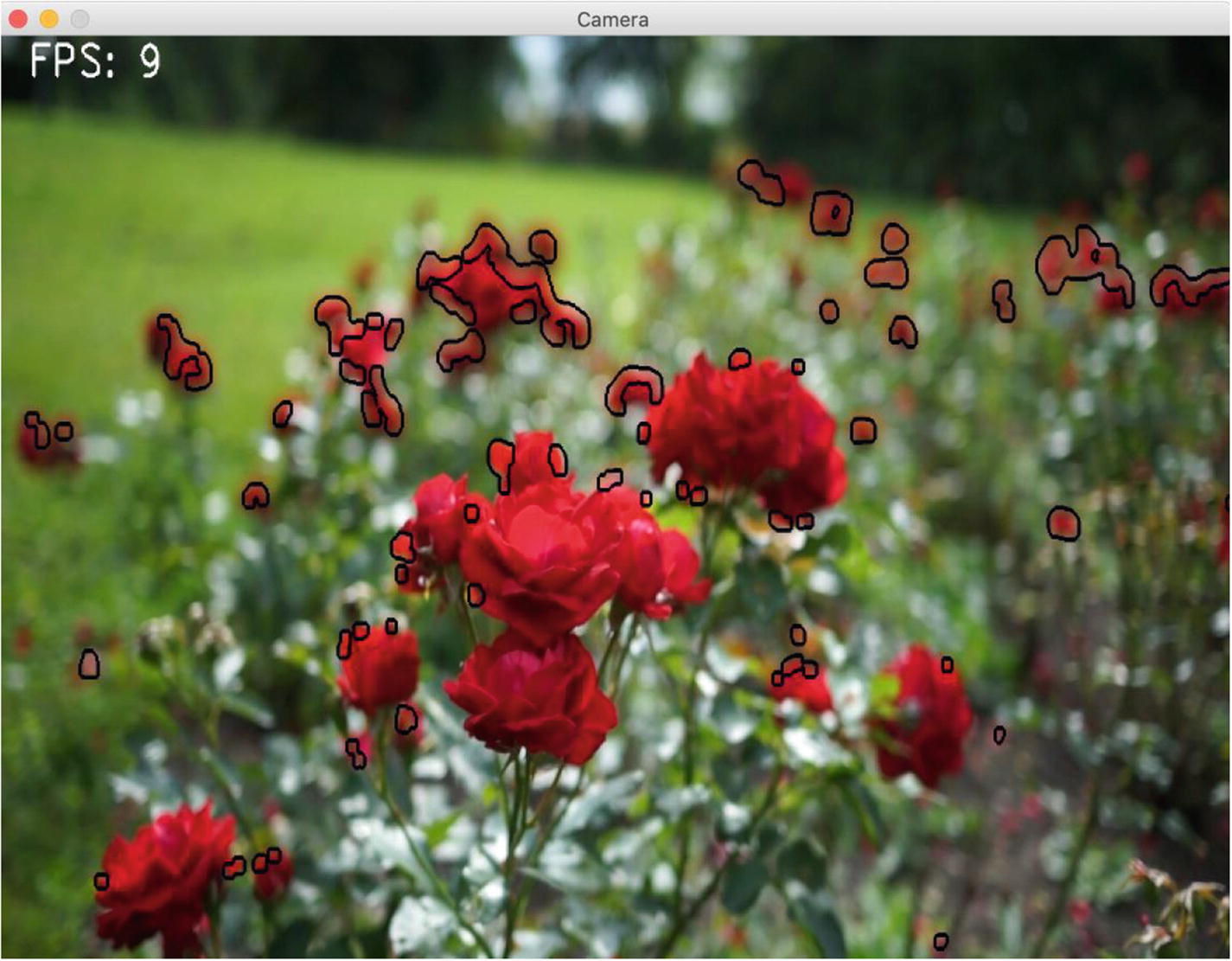
Detecting red roses
Looking at the values for Hue in Table 4-1, you can see it would not be so difficult to implement a filter that searches for blue colors. This is left as an exercise for you.
Detecting by Haar
As you saw in Chapter 1, you can use a Haar-based classifier to identify objects and/or people in a Mat object. The code is pretty much the same as you have seen, with an added emphasis on the number and size of shapes we are looking for.
Haar Classifier–Based Detection
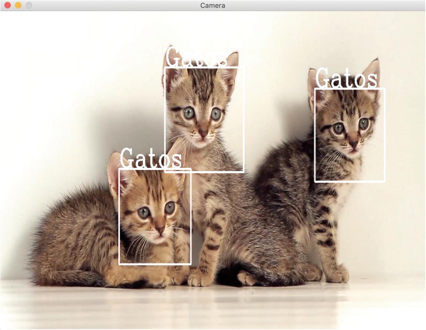
Finding cats
There are other XML files for Haar cascades in the samples. Feel free to use one to detect people, eyes, or smiling faces as an exercise.
Transparent Overlay on Detection
When drawing the rectangles in the previous examples, you might have wondered whether it is possible to draw something other than rectangles on the detected shapes.
Listing 4-18 shows how to do this by loading a mask that will be overlaid at the location of the detected shape. This is pretty much what you use in your smartphone applications all the time.
Note that there is a trick here with the transparency layer in the drawTransparency function. The mask for the overlay is loaded using IMREAD_UNCHANGED as the loading flag; you have to use this or the transparency layer is lost.
Adding an Overlay
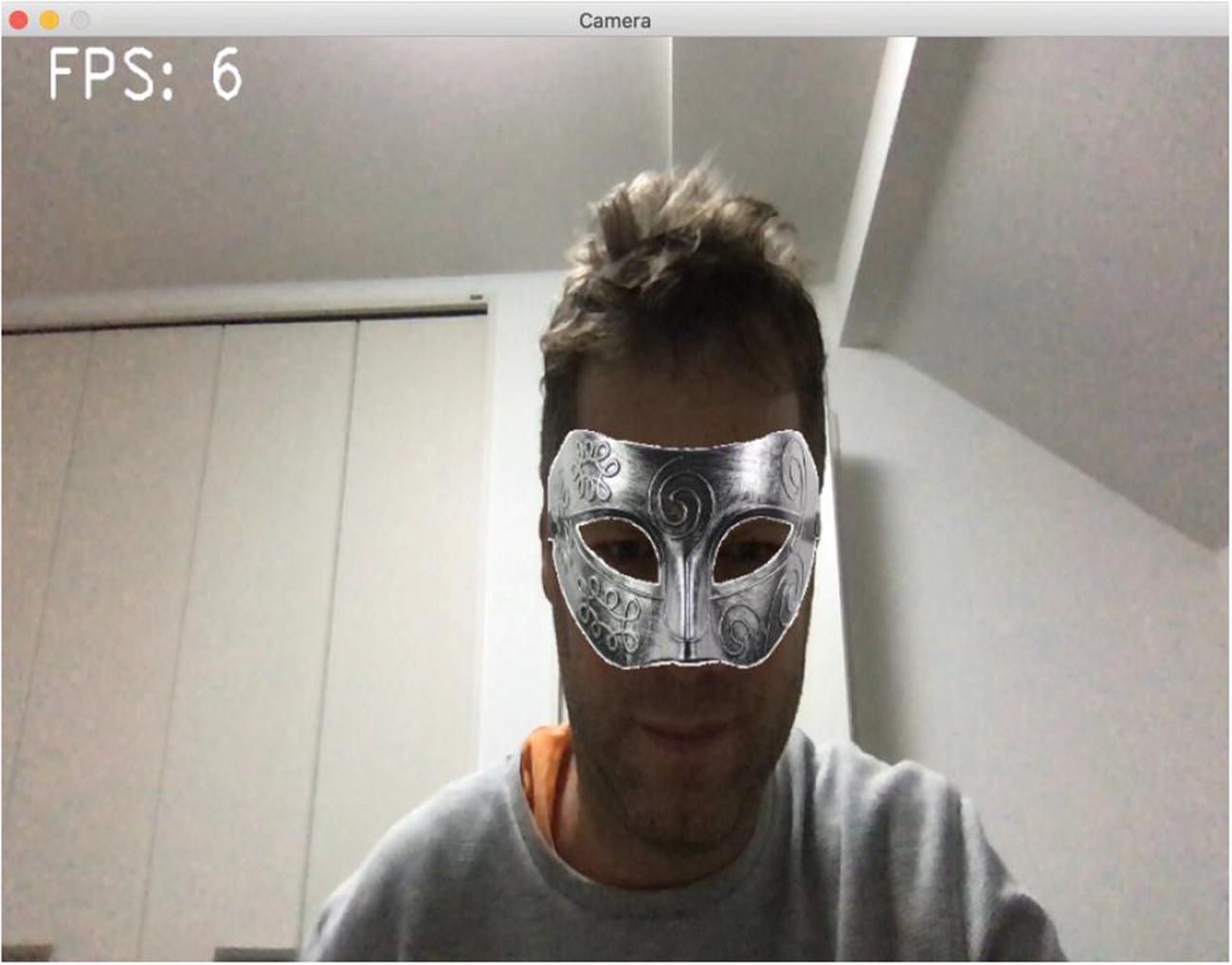
Adding a mysterious mask as an overlay
I actually tried and could not find a proper Batman mask to use as an overlay to the video stream. Maybe you can help me by sending me the code with an appropriate Mat overlay to use!
Detecting by Template Matching
Template matching with OpenCV is just plain simple. It’s so simple that this should maybe have come earlier in the order of detection methods. Template matching means looking for a Mat within another Mat. OpenCV has a superpower function named matchTemplate that does this.
Pattern Matching
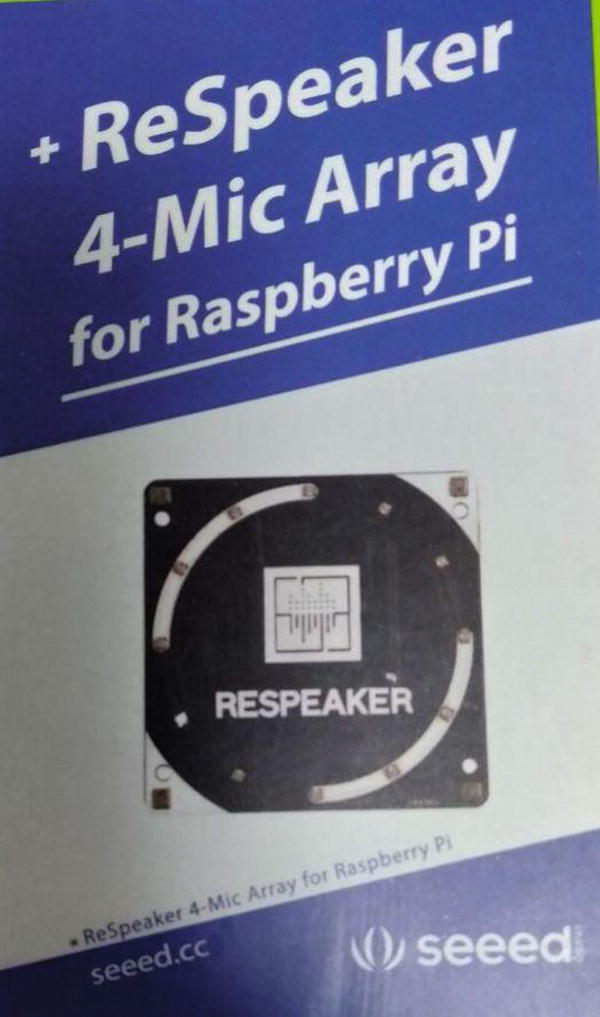
The template
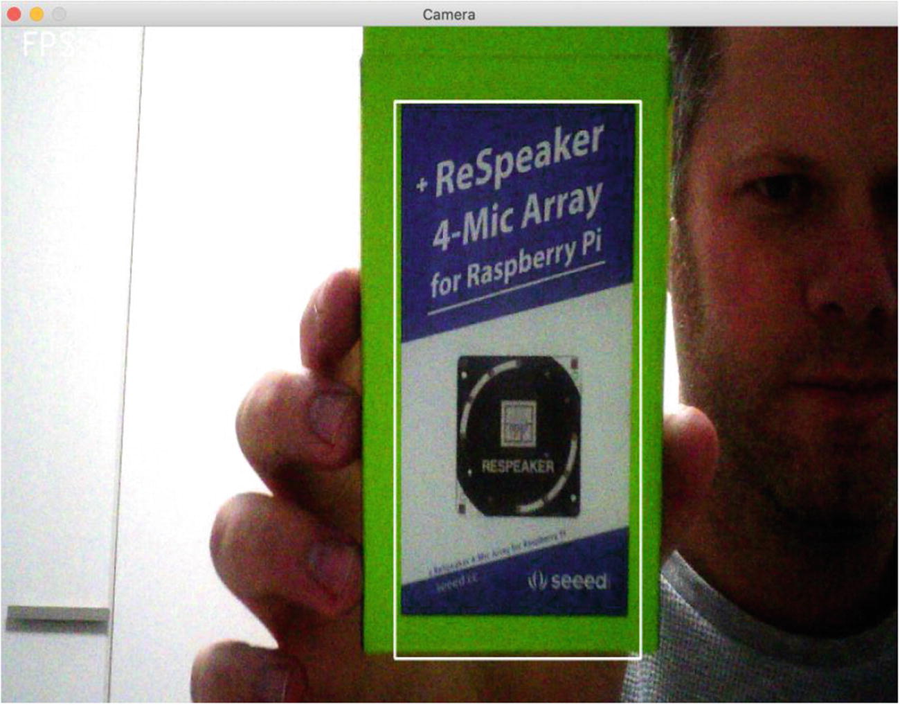
Finding the box for the speaker
It’s a bit hard to see the frame rate in Figure 4-18, but it is actually around 10 to 15 frames per second on the Raspberry Pi 4.
Detecting by Yolo
This is the final detection method presented in this chapter. Let’s say we want to apply a trained neural network to identify objects in a stream. After some testing on the hardware with little computing power, I got quite speedy results with Yolo/Darknet and the freely available Darknet networks trained on the Coco dataset.
The advantage of using neural networks on random inputs is that most of the trained networks are quite resilient and give good results, with 80 percent to 90 percent accuracy on close to real-time streams.
Training is the hardest part of using neural networks. In this book, we’ll restrict ourselves to running detection code on the Raspberry Pi, not training. You can find the steps for how to organize your pictures for re-training networks on the Darknet/Yolo web site.
- 1.
Load a network from its configuration file and weight file.
- 2.
Find the output layers/nodes of that network, because this is where the results will be. The output layers are the layers that are not connected to more output layers.
- 3.
Transform a Mat object into a blob for the network. A blob is an image, or a set of images, tuned to match the format expected by the network in terms of size, channel orders, etc.
- 4.
We then run the network, meaning we feed it the blob and retrieve the values for the layers marked as output layers.
- 5.
For each line in the results, we actually get a confidence value for each of the expected possible recognizable features. In Coco, the network is trained to be able to recognize 80 different possible objects, such as people, bicycles, cars, etc.
- 6.
We then use MinMaxLocResult again to get the index for the most probable recognized object, and if the value for that index is more than 0, we keep it.
- 7.
The first four values in each result line are actually the four values describing a box where the detected object was found, so we extract those four values and keep the rectangle and the index for its label.
- 8.
Before drawing all the boxes, we also usually make use of NMSBoxes, which removes overlapping boxes. Most of the time overlapping boxes are multiple versions of the same positive detection on the same object.
- 9.
Finally, we draw the remaining rectangle and add the label for the recognized object.
Neural Network –Based Detection
Java Classes and Constructors for the Different Yolo Networks
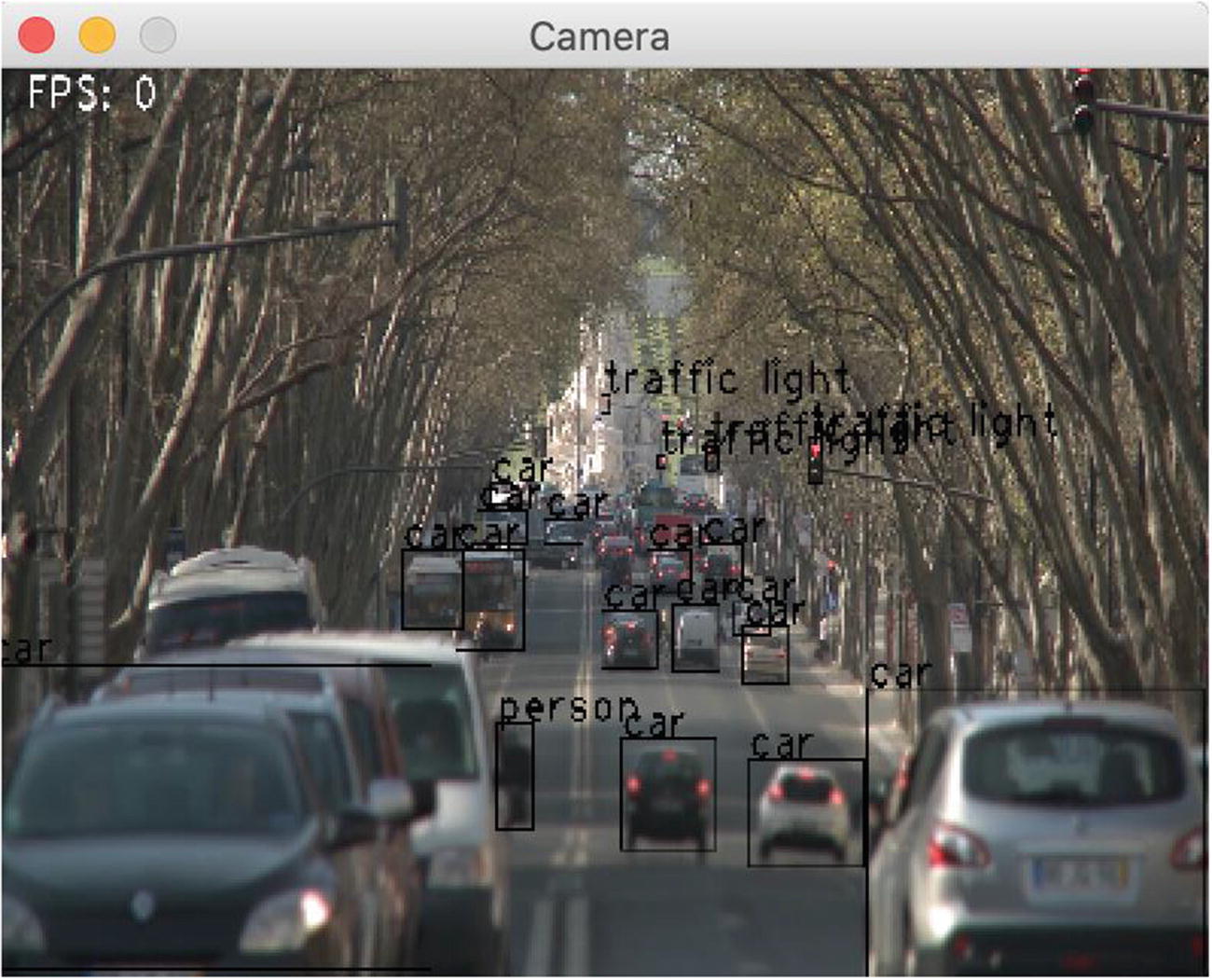
Yolo v3 detecting cars and people
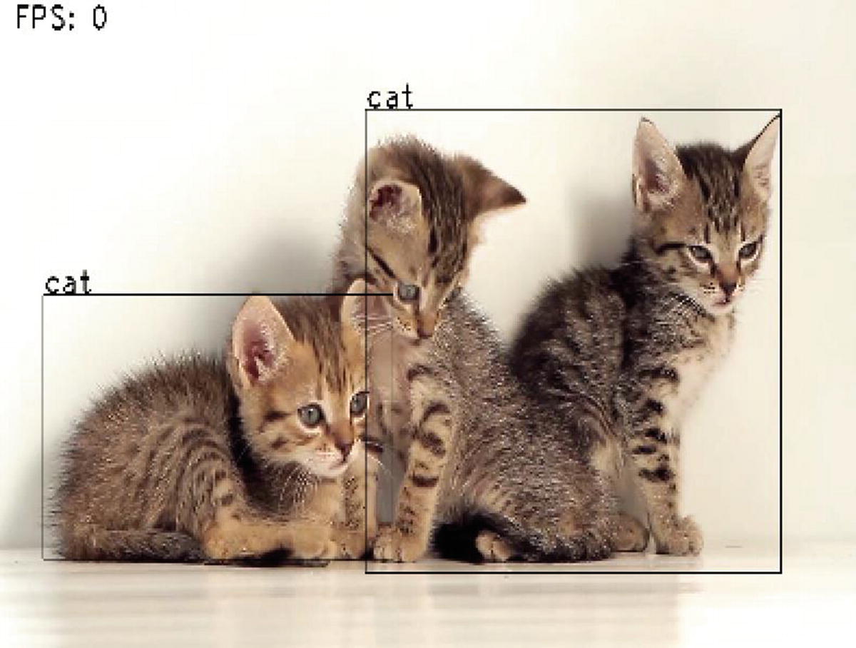
Yolo v3 detecting cats
As you can see, the frame rate was actually very low for standard Yolo v3.
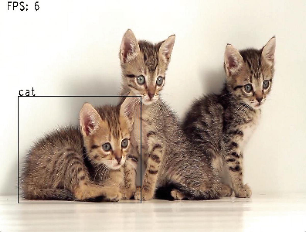
TinyYoloV3 detecting cats
You know my method. It is founded upon the observation of trifles.
—Arthur Conan Doyle,“The Boscombe Valley Mystery” (1891)
You’re down to the last few lines of this chapter, and it has been a long ride where you saw most of the object detection concepts with OpenCV in Java on the Raspberry Pi.
How to set up the Raspberry Pi for real-time object detection programming
How to use filters and pipelines to perform image and real-time video processing
How to implement some basic filters for Mat, used directly on real-time video streams from external devices and file-based videos
How to add some fun with Instagram-like filters
How to implement numerous object detection techniques using filters and pipelines
How to run a neural network trained on the Coco dataset that can be used in real time on the Raspberry Pi
In the next chapter, you’ll be introduced to Rhasspy, a voice recognition system, to connect the concepts presented in this chapter and apply them to home, office, or cat house automation.