Abercrombie & Fitch and Jewelry Sales Regression Case Studies1
Case I: Abercrombie & Fitch Sales in the United States
The Family Clothing Store industry, in which Abercrombie & Fitch Co. (A&F) operates, is highly fragmented and is dominated by a large number of small retailers, each with a low market share of the total industry. The top four players in this industry are A&F, Gap Inc., American Eagle Outfitters, Inc., and Ross Stores. These four companies collectively account for about 40 percent of the market. A&F generally charges higher prices compared with similar merchandise at Gap and American Eagle. The company was founded in 1892 and is headquartered in New Albany, Ohio.
The Company’s stores offer knit and woven shirts, graphic t-shirts, fleece, jeans and woven pants, shorts, sweaters, and outerwear. A&F operates more than one thousand stores in the United States, Canada, and the United Kingdom. It also sells its products through the Internet and catalogues.
The A&F brand targets college students. The RUEHL Brand, launched in 2005 and dropped in 2008, was a mix of business casual and trendy fashion, created to appeal to the modern-minded and post-college customers. In early 2007, the company launched another brand, Gilly Hicks, which specializes in women’s underwear, sleepwear, personal care products, and at-home products. This line was dropped at the start of 2014.
The Data
To build a regression model for sales of A&F the dependent variable is sales of A&F on a quarterly basis and in thousands of dollars.2 These values are shown in Figure 10.1 as a time-series plot constructed in Excel. As you see, sales increased from the beginning of this series until the economic downturn in 2008. After the economic downturn sales picked up again until 2013.
You also see sharp peaks that may represent seasonality in their sales. For A&F, the fiscal year runs from February to January, which makes February, March, and April the first quarter and subsequently November, December, and January the last quarter. The data are labeled using the middle month of the quarter. Thus, March represents the first quarter and December represents the fourth quarter of each year.
When you think about constructing a model for a company’s sales one of the first things that comes to mind is some measure of consumer buying power. You may know the concept of a “normal good.” The products sold by A&F would be considered normal goods. A normal good is one for which sales would increase as income increases. For this example, personal income (PI) in billions of dollars is used as a measure of buying power.
Unemployment often affects retail sales beyond the effect that unemployment has on income. If consumers are unemployed, or if they are employed but have concerns about losing their jobs, their purchasing behavior is likely to change. In the case of A&F the clothing and other items they sell would be considered discretionary goods. Thus, in times of high unemployment, consumers may put off purchases from a store such as A&F.
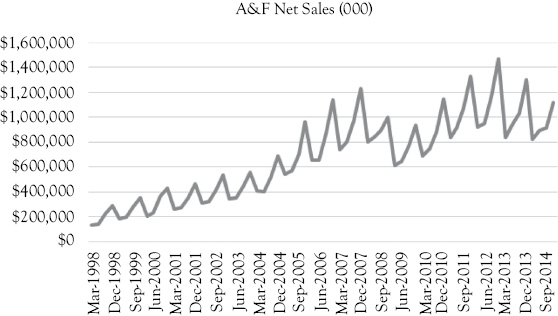
Figure 10.1 Abercrombie & Fitch sales (in 1000s of $)
Most retail sales have considerable seasonality. You can see this in Figure 10.1. Therefore, you would want to use dummy variables to evaluate the degree and nature of seasonality.
During the period considered A&F launched two new brands. One was the “RUEHL” brand and the other was “Gilly Hicks.” For each brand you could create a dummy variable with a one when that brand existed and zero otherwise. The RUEHL brand was only on the market from 2005 through 2007; so the dummy variable for RUEHL is a one in the 12 quarters covering 2005 through 2007. The other brand, Gilly Hicks, was started in early 2007 and was dropped at the start of 2014. The dummy variable for Gilly Hicks is therefore a one starting in the first quarter of 2007 through the end of 2013, and zero in all other periods.
The Hypotheses
When you do a regression analysis you should think carefully about the expectations you have for each independent variable. Do you expect a positive or negative coefficient for each of the independent variables? For the A&F regression model you have the following potential independent variables: personal income (PI), the unemployment rate (UR), seasonal dummy variables (Q1, Q2, Q3, and Q4), RUEHL brand, and Gilly Hicks brand. Thus, you should think about the direction of the impact each of these could have on A&F sales.
Hypothesis 1. The Expected Influence of Income
When the personal income of individuals increase, they tend to purchase more as their buying power increases. On the other hand, when the personal income falls, their purchasing power is reduced and they lower their purchases of normal goods. Thus, your research hypothesis is that the true regression slope (β) between sales and income should be positive. Thus, your hypotheses for personal income are:
H0 : β ≤ 0
H1 : β > 0
This form of the statistical test is appropriate for personal income, because you expect a direct relationship between sales of A&F and personal income. You expect an increase (decrease) in personal income to cause an increase (decrease) in A&F sales.
Hypothesis 2. The Expected Influence of the Unemployment Rate
You might expect that there is more than an income effect of unemployment on the sale of consumer goods. You would expect that the sales of A&F would have an inverse relationship with the unemployment rate. Thus, your hypotheses for the unemployment rate are:
H0 : β ≥ 0
H1 : β < 0
If the unemployment rate increases, then the A&F sales would be expected to decreases and vice versa.
Hypothesis 3. Seasonal Dummy Variables
You might expect that A&F would experience the greatest sales activity during the fall season due to the back-to-school sales as well as in the last part of the year due to holiday gift buying. The first quarter of the year is typically the lowest quarter for retail sales of almost all types of products. Thus, it makes sense to use the first quarter as the base period. As a result, you would expect sales to be higher in quarters two, three, and four than in the first quarter of each year. Thus, your hypotheses for Q2, Q3, and Q4 are all the same as follows:
H0 : β ≤ 0
H1 : β > 0
Hypothesis 4. RUEHL and Gilly Hicks
With regard to the dummy variables for the RUEHL and the Gilly Hicks brands, you would expect a positive relationship to overall sales. Remember that these two dummy variables are equal to 1 when the brand exists and equal to 0 when the brand does not exist. Thus the hypotheses for each of these brands (RUEHL and Gilly Hicks) would be:
H0 : β ≤ 0
H1 : β > 0
The Regression Models
To help you see the development of regression models, four models of A&F sales are discussed in this section. The first includes only one independent variable (personal income), the second adds unemployment, the third also includes seasonal dummy variables, and finally, the fourth model adds the two dummy variables related to the RUEHL and Gilly Hicks brands.
For each model you will see the Excel regression results and a graph of the actual A&F sales compared with the predictions from each model. You will also see a brief discussion of the five-step evaluation of each model. We do not show the ANOVA for each of the four models since the F-ratios are significant for all four at a 95 percent confidence level.
Model 1. Sales as a Function of Personal Income
First, look at the regression results from Excel in Table 10.1. As you see, the Excel regression output has been edited to help you concentrate on the most important parts of the tables. These results will form the basis for your five-step evaluation of the first model.
The most important statistical results are in bold in the Excel output in Table 10.1. From the Coefficients column you can write the equation for this model as:
Sales = –729,607.4 + 144.340 (PI)
Table 10.1 A&F sales as a function of personal income
|
S = f(PI) |
||||
|
Regression Statistics |
||||
|
R-square |
0.789 |
DW = 1.656 |
||
|
Adjusted R-square |
0.786 |
|||
|
Standard error |
153,886 |
|||
|
Observations |
68 |
|||
|
Coefficients |
t Stat |
P-Value |
P/2 |
|
|
Intercept |
–729,607.4 |
15.7085.7087.773 |
0.000 |
0.000 |
|
PI |
144.340 |
9.189 |
0.000 |
0.000 |
Step 1: Is the Model Logical?
You would expect that as consumers’ incomes increase A&F would sell more goods. Therefore, the positive (+) sign for the coefficient (slope) related to income is logical.
Step 2: Is the Slope Term Significantly Positive?
In order to check for statistical significance of the independent variable (PI) the hypothesis for the slope of income is subjected to a one-tailed t-test. If the absolute value of calculated tc is greater than the t-table value at the 95 percent confidence level (5 percent significance level), you can reject the null hypothesis. This means that you have empirical support for the research hypothesis. To determine the t-table value, the degree of freedom (df) is calculated as df = n – (k + 1). In this case, n = number of observations in the model = 68 and k = number of independent variables = 1. Thus, df = 68 – (1 + 1) = 66. The t-table value is approximately 1.671 (see Appendix 4B, and use the row for df=60, which is the closest value to 66).
The calculated t-ratio for disposable personal income is 9.189. This would be very far into the right tail of the distribution as indicated by a P-value of 0 to three decimal places. In the Excel output table, you see a column that is added for the p-value divided by two (P/2) because you would be doing a one-tailed test and the P-value provided by Excel is for both tails of the distribution. Of course, P/2 is also less than the desired level of significance of 0.05. Thus, there is very little risk of error in rejecting the null hypothesis.
Step 3: What is the Explanatory Power of the Model?
For this bivariate regression model, the explanatory power is measured by the coefficient of determination, R2. The coefficient of determination tells you the percentage of the variation in the dependent variable (A&F sales) that is explained by the one independent variable, personal income (PI). In this model, the coefficient of determination (R2) is 0.789, which means 78.9 percent of the variation in the A&F sales is explained by this model.
Step 4: Check for Serial Correlation
Because time-series data are used in this model you need to be concerned about possible serial correlation. You can evaluate this using the DW statistic. The DW statistic will always be in the range of 0–4 and as a rule of thumb, a value between 1.5 and 2.5 is suggestive that there may be no serial correlation.
The DW statistic for this model is 1.656. Based on the table in Appendix 4C and the discussion in Appendix 4D you see that du < 1.656 < 2, so Test 4 is satisfied and you can say that no serial correlation exists. For this case, you would use du = 1.544 with n = 40 and k = 1.3
Step 5: Check for Multicollinearity
For a simple model with only one independent variable there is no possible multicollinearity. In Figure 10.2, the graph shows the actual A&F sales (solid line) along with the predictions based on Model 1 (dotted line). What do you think is most clearly missing in the model?
Model 2. Sales as a Function of Personal Income and Unemployment Rate
Now we will expand Model 1 to include more variables in Models 2 through 4. Your evaluation of each model should follow the same format as for Model 1. Looking at three more models of sales for A&F will help you understand how models are developed and evaluated.
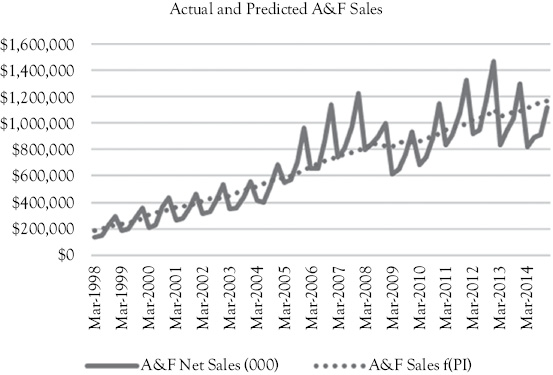
Figure 10.2 A&F actual sales (solid line) and predictions (dotted line) based on Model 1
Suppose that next you decide to add the unemployment rate as an additional independent variable. Again you should first look at the regression results from Excel shown in Table 10.2. Here PI = personal income and UR = unemployment rate.
The Excel results in Table 10.2 provide the basis for your five-step evaluation of the second model. The most important statistical results are in bold. From the Coefficients column you can write the equation for this model as:
Sales = –724,899.5 + 156.675 (PI) – 20,386.882 (UR)
Step 1: Is the Model Logical?
Again, you expect that as consumers’ incomes increase A&F would sell more goods so the positive (+) sign for the slope related to income is logical. And, you would expect that a higher unemployment would result in lower sales. Thus, the negative slope for UR is logical.
Step 2: Are the Slope Terms Significantly Positive?
Table 10.2 A&F sales as a function of personal income and the unemployment rate
|
S = f(PI,UR) |
||||
|
Regression Statistics |
||||
|
R-square |
0.796 |
DW = 1.708 |
||
|
Adjusted R-square |
0.789 |
|||
|
Standard error |
152,550 |
|||
|
Observations |
68 |
|||
|
Coefficients |
t Stat |
P-Value |
P/2 |
|
|
Intercept |
–724,899.5 |
–7.983 |
0.000 |
0.000 |
|
PI |
156.675 |
12.651 |
0.000 |
0.000 |
|
UR |
–20,386.882 |
–1.470 |
0.146 |
0.073 |
Now you need to evaluate each of the two slope terms. Since you now have two independent variables df = n – (k + 1) = 68 – (2 + 1) = 65. Because the closest value for df in your table is 60, you would again use a t-table value of 1.671. For personal income, the calculated t-statistics is well into the upper tail of the distribution. However, for the unemployment rate the calculated t is not out in the lower tail of the distribution. Further, only for income (PI) is P/2 is less than the level of significance of 0.05. This means that you have empirical support that income has a significant influence on A&E sales at a 95 percent confidence level. However, the P/2 value for the unemployment rate exceeds the 0.05 critical value so we cannot say the same for UR. We can say that unemployment has a significant affect on sales if we lower our confidence level to 90 percent, which is not uncommon (note that P/2 for UR is less than 0.10).
Step 3: What is the Explanatory Power of the Model?
For this multiple regression model, the explanatory power is measured by the coefficient of determination, but now you must use the adjusted R-square. This coefficient of determination tells you the percentage of the variation in the dependent variable (A&F sales) that is explained by PI and the UR. In this model, the coefficient of determination (adjusted R2) is 0.789, which means 78.9 percent of the variation in the A&F sales is explained by this model. This is essentially the same as for the bivariate model. The R-square is higher for this model but because we have lost one degree of freedom it turns out that the adjusted R-square is the same as the R-square for the bivariate model.
Step 4: Check for Serial Correlation
Again you need to be concerned about possible serial correlation. The DW statistic for this model is 1.708. Based on the table in Appendix 4C and the discussion in Appendix 4D you see that 1.600 < 1.708 < 2, so Test 4 is satisfied and you can say that no serial correlation exists. For this case, you would use du = 1.600 with n = 40 (rather than n = 68) and k = 2.
Step 5: Check for Multicollinearity
With more than one independent variable you need to look at the correlation matrix for all pairs of independent variables. The correlation between PI and UR is 0.68, so the two variables are not strongly enough correlated to cause a problem. Also, there is no indication in the model of a multicollinearity problem, since both signs for coefficients are as you expect.
In Figure 10.3, you see a graph that shows the actual A&F sales (solid line) along with the predictions based on Model 2 (dotted line). This model fits a bit better than Model 1 but it is not as good as you would hope. What do you think is still missing?
Model 3. Sales as a Function of PI, UR, and Two Seasonal Dummy Variables (Q3 and Q4)
Having recognized that both Models 1 and 2 failed to account for the seasonal variation in A&F sales, you would naturally try to add seasonal dummy variables. Analysis of the data shows that there is only significant seasonality during the back to school and holiday seasons (quarters Q3 and Q4). Therefore, you only need seasonal dummy variables for these two quarters of each year.
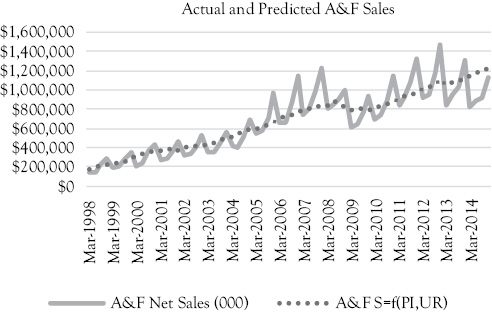
Figure 10.3 A&F actual sales (solid line) and predictions (dotted line) based on Model 2
You rely upon the regression results from Excel as shown in Table 10.3 to evaluate Model 3. Here PI = personal income, and UR = the unemployment rate, while Q3 and Q4 represent the corresponding quarters. From the Coefficients column, you can write the equation for this model as:
Sales = – 794,137.7 + 152.208 (PI) – 1t7,766.012 (UR) + 110,692.074 (Q3) + 276,248.649 (Q4)
Step 1: Is the Model Logical?
Again, you expect that as consumers’ incomes increase A&F would sell more goods and as unemployment increases they would be expected to sell less. Thus, a positive sign for the slope related to income is logical as is the negative sign for unemployment. You would expect quarters Q3 and Q4 to have higher sales than the rest of the year due to back to school and holiday shopping. Q3 is a dummy variable equal to 1 every third quarter and 0 otherwise. Q4 is a dummy variable equal to 1 every fourth quarter and 0 otherwise. Thus, the positive coefficients for Q3 and Q4 make sense.
Table 10.3 A&F sales as a function of personal income, the unemployment rate, and seasonal dummy variables for Q3 and Q4
|
S = f(PI,UR,Q3,Q4) |
||||
|
Regression Statistics |
||||
|
R-square |
0.913 |
DW = 0.737 |
||
|
Adjusted R-square |
0.907 |
|||
|
Standard error |
101,302 |
|||
|
Observations |
68 |
|||
|
Coefficients |
t Stat |
P-Value |
P/2 |
|
|
Intercept |
–794,137.7 |
–13.012 |
0.000 |
0.000 |
|
PI |
152.208 |
18.474 |
0.000 |
0.000 |
|
UR |
–17,766.012 |
–1.928 |
0.058 |
0.029 |
|
Q3(Aug–Oct) |
110,692.074 |
3.676 |
0.000 |
0.000 |
|
Q4(Nov–Jan) |
276,248.649 |
9.164 |
0.000 |
0.000 |
Step 2: Are the Slope Terms Significantly Positive?
Now you need to evaluate all four slope terms. Since you now have four independent variables, df = n – (k + 1) = 68 – (4 + 1) = 63. Again you would use a t-table value of 1.671. For all four variables, the calculated t-statistics are well into the tails of the distribution (the upper tail for PI, Q3, Q4, and the lower tail for UR). Further, in all cases P/2 is less than the desired level of significance of 0.05. This means that you have empirical support for all four of the research hypotheses (at greater than a 95 percent confidence level).
Step 3: What is the Explanatory Power of the Model?
For this multiple regression model, the explanatory power is again measured by the adjusted R-square. This value tells you the percentage of the variation in the dependent variable (A&F sales) that is explained by PI, UR, and seasonality as measured by Q3 and Q4. In this model, the adjusted R-square is 0.907, which means 90.7 percent of the variation in the A&F sales is explained by this model. This is a big improvement and helps you to see the importance of seasonality as measured by using dummy variables for seasonality.
Step 4: Check for Serial Correlation
Again you need to be concerned about possible serial correlation. The DW statistic for this model is 0.737. Based on the table in Appendix 4C and the discussion in Appendix 4D, you see that 0 < 0.737 < dl = 1.285 so Test 6 is satisfied, which means that this model has a positive serial correlation problem. This means that standard errors may be underestimated and thus t-ratios may be larger than they should be and some null hypotheses may have been incorrectly rejected in favor of the research hypotheses. Given the sizes of the t-ratios calculated, this is most likely to be a problem related to unemployment rather than the other independent variables, since the other t-ratios are very large. One solution may be that you are missing some useful causal (independent) variables.
Step 5: Check for Multicollinearity
With more than one independent variable, you need to look at the correlation matrix for all pairs of independent variables. The correlation matrix is shown in Table 10.4. The correlations between the individual pairs of independent variables in this model are not very high as shown in the correlation matrix in Table 10.4. Also, there is no indication in the model of a multicollinearity problem, since the signs for all four coefficients are as you expect.
In Figure 10.4, you see a graph that shows the actual A&F sales (solid line) along with the predictions based on Model 3 (dotted line). This model fits much better than Model 2 but has a positive serial correlation issue.
Model 4. Sales as a Function of Personal Income, Unemployment Rate, Two Seasonal Dummy Variables (Q3 and Q4), and Dummy Variables for Two Brands
During the period for which data have been used, A&F added the RUEHL brand in 2005 then dropped it in 2008. They added the Gilly Hicks brand in 2007, but dropped that brand in 2014. For each quarter in the data, the RUEHL and the Gilly Hicks brands either were or were not part of A&F. Thus, you can create a dummy variable for each brand that equals 1 when the brand was active and 0 otherwise.
Let us now look at one more regression model. In this last model we will include PI, UR, Q3, Q4, the RUEHL brand, and the Gilly Hicks brand as independent variables.
Table 10.4 Correlation matrix for personal income (PI), the unemployment rate (UR), and seasonal dummy variables for Q3 and Q4
|
PI |
UR |
Q3(Aug–Oct) |
Q4(Nov–Jan) |
|
|
PI |
1.000 |
|||
|
UR |
0.68 |
1.000 |
||
|
Q3 (Aug–Oct) |
0.02 |
0.01 |
1.000 |
|
|
Q4 (Nov–Jan) |
0.04 |
0.01 |
–0.33 |
1.000 |
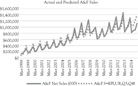
Figure 10.4 A&F actual sales (solid line) and predictions (dotted line) based on Model 3
These results, as shown in Table 10.5, form the basis for your Five-step evaluation of the fourth (and last) model. From the Coefficients column you can write this equation as:
Sales = - 641,007.4 + 125.007 (PI) - 13,720.666 (UR) + 114,806.255 (Q3) + 282,904.094 (Q4) + 147,302.158 (R) + 142,508.792 (GH)
Step 1: Is the Model Logical?
Again, you expect that A&F would sell more goods as PI increases, when it is a third or fourth quarter and when they have the RUEHL and Gilly Hicks brands. You would expect them to have lower sales if unemployment increases. Therefore, all six slope terms in the model have signs for their coefficients that make sense.
Step 2: Are the Slope Terms Significantly Positive?
Now you need to evaluate all six slope terms. Now that you have six independent variables, df = n – (k + 1) = 68 – (6 + 1) = 61. Again you would use a t-table value of 1.671. For five of the six independent variables the calculated t-statistics are well into the tails of the distribution (the upper tail for PI, Q3, Q4, RUEHL, and Gilly Hicks). For the unemployment rate (UR), the calculated t-ratio of -1.642 is slightly less negative than the t-table value of -1.671. Certainly all six independent variables would have a significant impact on A&F sales at a 90 percent confidence level, which is also commonly used. It is likely that an analyst would leave all six of the current independent variables in the model. This is especially true since the P/2 value for unemployment is 0.053.
Table 10.5 A&F sales as a function of personal income, the unemployment rate, seasonal dummy variables for Q3 and Q4, and dummy variables for the RUEHL and Gilly Hicks brands
|
S = f(PI,UR,Q3,Q4,R,GH) |
||||
|
Regression Statistics |
||||
|
R-square |
0.958 |
DW = 1.492 |
||
|
Adjusted R-square |
0.954 |
|||
|
Standard error |
71,332 |
|||
|
Observations |
68 |
|||
|
Coefficients |
t Stat |
p-Value |
P/2 |
|
|
Intercept |
–641,007.4 |
–11.544 |
0.000 |
0.000 |
|
PI |
125.007 |
18.644 |
0.000 |
0.000 |
|
UR |
–13,720.666 |
–1.642 |
0.106 |
0.053 |
|
Q3(Aug–Oct) |
114,806.255 |
5.413 |
0.000 |
0.000 |
|
Q4(Nov–Jan) |
282,904.094 |
13.316 |
0.000 |
0.000 |
|
RUEHL Brand |
147,302.158 |
5.586 |
0.000 |
0.000 |
|
Gilly Hicks Brand |
142,508.792 |
5.174 |
0.000 |
0.000 |
This means that there is strong statistical support for the positive influence of personal income, quarter 3, quarter 4, the RUEHL brand and the Gilly Hicks brand on sales revenue for A&E. There is some support for a negative affect of the unemployment rate on sales, but the statistical support is not as strong as for the other causal variables.
Step 3: What is the Explanatory Power of the Model?
For this multiple regression model, the explanatory power is again measured by the adjusted R2. In this model the adjusted R2 is 0.954, which means 95.4 percent of the variation in the A&F sales is explained by PI, UR, seasonality, and the existence of the RUEHL and Gilly Hicks brands. This is an improvement over Model 3.
Step 4: Check for Serial Correlation
Again you need to be concerned about possible serial correlation. The DW statistic for this model is 1.492. Based on the table in Appendix 4C and the discussion in Appendix 4D you see that dl = 1.175 < 1.492 < du = 1.854 (n = 40 and k = 6).
Test 3 is satisfied This means that the test for serial correlation is indeterminate.4 By adding two additional variables that have a significant effect on A&F sales has alleviated the potential serial correlation that you observed in Model 3.
Step 5: Check for Multicollinearity
You know that with more than one independent variable you need to look at the correlation matrix for all pairs of independent variables. The correlations between the individual pairs of independent variables in this model are not very high as shown by the correlation matrix below in Table 10.6. Also, there is no indication in the model of a multicollinearity problem, since the signs for all four coefficients are as you expect.
Table 10.6 Correlation matrix for personal income (PI), the unemployment rate(UR), seasonal dummy variables for Q3 and Q4, and dummy variables for RUEHL and Gilly Hicks
|
PI |
UR |
Q3 (Aug–Oct) |
Q4 (Nov–Jan) |
RUEHL brand |
Gilly Hicks brand |
|
|
PI |
1.00 |
|||||
|
UR |
0.68 |
1.00 |
||||
|
Q3(Aug–Oct) |
0.02 |
0.01 |
1.00 |
|||
|
Q4(Nov–Jan) |
0.04 |
0.01 |
-0.33 |
1.00 |
||
|
RUEHL brand |
0.03 |
-0.35 |
0.00 |
0.00 |
1.00 |
|
|
Gilly Hicks brand |
0.69 |
0.71 |
0.00 |
0.00 |
-0.07 |
1.00 |
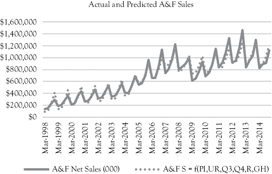
Figure 10.5 A&F actual sales (solid line) and predictions (dotted line) based on Model 4
In Figure 10.5, you see a graph that shows the actual A&F sales (solid line) along with the predictions based on Model 4 (dotted line). This model fits very well and does not have a positive serial correlation problem.
Case II: Retail Jewelry Sales in the United States
This case involves the total sales of jewelry stores in the United States (U.S. Retail Sales: Jewelry Stores. NAICS 44831, in millions of dollars. Source: economagic.com). The original data were on a monthly basis, however to simplify the number of dummy variables needed to deal with seasonality the data have been transformed to a quarterly basis. See Figure 10.6.
In Figure 10.6 you see that jewelry sales have generally been increasing over the period used for this example (the first quarter of 2004 through the last quarter of 2014). There was a drop during 2008 when the U.S. economy had a general downturn that affected most economic activity.
Model 1. Jewelry Sales as a Function of Disposable Personal Income Per Capita
We will build a series of regression models to help you see how one can evaluate models working toward a model that is appropriate for the analyst’s use. For a product such as jewelry sales one of the first variables one might think of is a measure of consumer buying power. For this purpose we have selected disposable personal income per capita (DPIPC). This measure of income is the average amount people earn in one year in the United States.
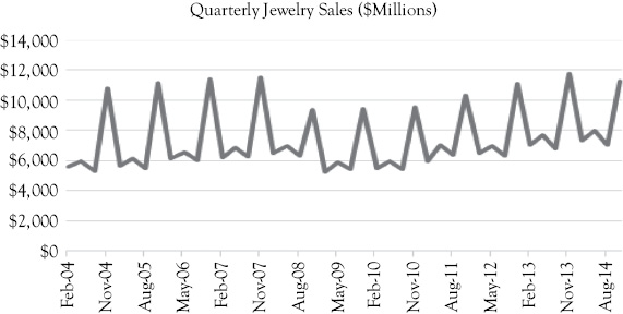
Figure 10.6 U.S. Jewelry Store Sales. Quarterly data show the seasonality and trend in jewelry sales
As we look at several models for jewelry sales we will go through the five step evaluation process that you have seen in previous examples. The regression results for the first model of jewelry sales (JS) as a function of disposable personal income per capita (DPIPC) are shown in Table 10.7.
Look at the regression results from Excel in Table 10.7. The Excel regression output has been edited to help you concentrate on the most important parts of the table which are in bold. From the Coefficients column you can write the equation for this model as:
JS = 1,333.545 + 0.169 (DPIPC)
Step 1: Is the Model Logical?
One would expect that jewelry sales would be positively related to how much money people have to spend. Therefore, the positive sign of the slope for DPIPC makes sense from an economic/business perspective.
Table 10.7 Jewelry sales (JS) as a function of purchasing power as measured by disposable personal income per capita (DPIPC)
|
Regression Statistics |
|||||
|
R Square |
0.065 |
DW = 2.637 |
|
||
|
Standard Error |
2007.228 |
|
|||
|
Observations |
44 |
|
|||
|
|
|||||
|
|
Coefficients |
Standard Error |
t Stat |
P-value |
P/2 |
|
Intercept |
1333.545 |
3560.528 |
0.375 |
0.710 |
0.355 |
|
DPIPC |
0.169 |
0.098 |
1.711 |
0.094 |
0.047 |
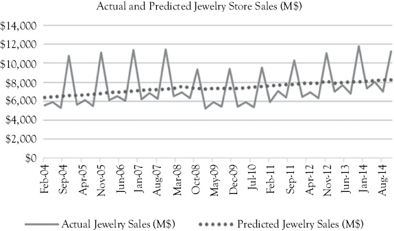
Figure 10.7 Jewelry sales as a function of disposable personal income per capita. The solid line represents actual sales while the dotted line is for the predicted values
The dotted regression line in Figure 10.7 follows the general upward trend in jewelry sales but has two things that you will recognize as being not quite what one might expect. First, the model fails to account for the seasonality in the data. We know this can be helped by using seasonal dummy variables which we will do shortly. Also, notice that during the economic downturn of 2008 the regression line does not seem to drop off as much as one might expect. We will address this in our second model. First, let us continue with the evaluation of the current regression model (JS = f(DPIPC)).
Step 2: Is the Slope Term Significantly Positive?
In order to check for statistical significance of the independent variable (DPIPC) the hypothesis for the slope of income is subjected to a one-tailed t-test. If the absolute value of calculated tc is greater than the t-table value at the 95 percent confidence level (5 percent significance level), you can reject the null hypothesis that the relation between JS and DPIPC is not positive.
H0 : β ≤ 0
H1 : β > 0
This would mean that you have empirical support for the research hypothesis that there is a positive relation between JS and DPIPC.
To determine the t-table value, the degree of freedom (df) is calculated as df = n – (k + 1). In this case, n = number of observations in the model = 44 and k = number of independent variables = 1. Thus, df = 44 – (1 + 1) = 42. The t-table value is approximately 1.684 (see Appendix 4B, and use the row for df = 40, which is the closest value to 42).
The calculated t-ratio for disposable personal income is 1.711. Would this would be in the right tail of the distribution? The answer is “Yes” because 1.711 is greater than 1.684. We see that the p-value is 0.094, which is greater than 0.05 – our desired significance level. However, the default t- statistic in Excel output is for a two tailed test. Thus, we need to divide that value by two since we are doing a one tailed test.
In the Excel output table, you see a column for the p-value divided by two (p/2). Here, p-value/2 is 0.047 and is less than the desired level of significance of 0.05. Thus, there we can reject the null hypothesis and conclude that we have evidence of a positive relationship between jewelry sales (JS) and income (DPIPC).
Step 3: What is the Explanatory Power of the Model?
For this bivariate regression model, the explanatory power is measured by the coefficient of determination, R2. In this model, the coefficient of determination (R2) is 0.065, which means 6.5 percent of the variation in the JS sales is explained by DPIPC. This may seem a small amount of explanatory power, but keep in mind we have just one independent variable at this point and we have not yet dealt with the pronounced seasonality in JS.
Step 4: Check for Serial Correlation
Because time-series data are used in this model you need to be concerned about possible serial correlation. The DW statistic for this model is 2.637. For this case, you would use dl = 1.442 and du = 1.544 with n = 40 and k = 1. Based on the table in Appendix 4C and the discussion in Appendix 4D you see that 4 - dl < 2.637 < 4, so Test 1 is satisfied and therefore this model has negative serial correlation. For now we will not worry about this result but it does signal to us to watch for serial correlation as we continue to develop the model.
Step 5: Check for Multicollinearity
For a simple model with only one independent variable there is no possible multicollinearity.
Model 2. Jewelry Sales as a Function of Disposable Personal Income Per Capita (DPIPC) and the Unemployment Rate (UR).
In Figure 10.7 we saw that when the only independent variable was DPIPC the regression predictions did not seem to account very well for the economic downturn in 2008. This suggests that we might want to include another variable that might account for a different dimension of the economic slump. We will consider the unemployment rate (UR) in this regard. So we will now have the following model:
JS = f (DPIPC, UR)
The statistical results for this model are in Table 10.8.
Step 1: Is the Model Logical?
One would still expect that jewelry sales would be positively related to how much money people have to spend. Therefore, the positive sign of the slope for DPIPC makes sense from an economic/business perspective. For the unemployment rate we might expect a negative relationship to jewelry sales because jewelry sales are generally something that could be delayed when consumers are worried about their employment situations. Thus, the negative coefficient for UR is logical. The regression equation is:
Table 10.8 Jewelry sales (JS) as a function of disposable personal income per capita (DPIPC) and the unemployment Rate (UR)
|
Regression Statistics |
|
|
|
|
|
|
R Square |
0.127 |
DW = 2.816 |
|
||
|
Adjusted R Square |
0.084 |
|
|||
|
Standard Error |
1963.186 |
|
|||
|
Observations |
44 |
|
|||
|
|
|||||
|
|
Coefficients |
Standard Error |
t Stat |
P-value |
p/2 |
|
Intercept |
441.836 |
3521.477 |
0.125 |
0.901 |
0.450 |
|
DPIPC |
0.251 |
0.108 |
2.330 |
0.025 |
0.012 |
|
UR |
-306.763 |
179.964 |
-1.705 |
0.096 |
0.048 |
JS = 441.836 + 0.251 (DPIPC) – 306.763 (UR).
The actual JS data and the regression line for Model 2 are graphed in Figure 10.8. The dotted regression line in Figure 10.8 follows the downturn in sales better than the results from Model 1 had done.
Step 2: Are the Slope Terms Significantly Positive or Negative?
Once more the hypothesis for DPIPC is:
H0 : β ≤ 0
H1 : β > 0
For the unemployment rate the hypothesis is:
H0 : β ≥ 0
H1 : β < 0
This is because our research hypothesis is that there would be a negative relationship between JS and UR.
To determine the t-table value, the degree of freedom (df) is still calculated as df = n – (k + 1). In this case, n = 44 and k = 2. Thus, df = 44 – (1 + 2) = 41. The t-table value is approximately 1.684 (see Appendix 4B, and use the row for df = 40, which is the closest value to 41).
The calculated t-ratio for disposable personal income is 2.330. This would be in the right tail of the distribution as indicated by a P-value of 0.025, and P/2 of 0.012. Notice that when UR is added to the model the t-statistic for DPIPC is higher than when only DPIPC is in the model. We see that the risk of error in rejecting the null hypothesis for DPIPC is low.
The calculated t-ratio for the unemployment rate is -1.705 which is more negative than the table value of –1.684. Correspondingly, you see that P/2 is 0.048 which is less than 0.05. Thus, we have empirical support that there is a negative relation between JS and UR.
Step 3: What is the Explanatory Power of the Model?
For this multiple regression model, the explanatory power is measured by the coefficient of determination, now the adjusted R2. In this model, the adjusted R2 is 0.084, which means 8.4 percent of the variation in the JS sales is explained by DPIPC. This may still seem a small amount of explanatory power, but it is more than when only income was considered. Keep in mind we not yet dealt with the pronounced seasonality in JS.
Step 4: Check for Serial Correlation
The DW statistic for this model is 2.816. For this case, you would use dl = 1.391 and du = 1.600 with n = 40 and k = 2. Based on the table in Appendix 4C and the discussion in Appendix 4D you see that 4 - dl < 2.816 < 4, so Test 1 is again satisfied and therefore this model also has negative serial correlation.
Step 5: Check for Multicollinearity
For a multiple regression model we need to consider whether or not there may be multicollinearity. To check for this we look at the bivariate correlations between all pairs of independent variables. This is shown in Table 10.9. We see that the correlation between income (DPIPC) and the unemployment rate (UR) is only 0.45 which is not high enough to suggest a great degree of overlap between the two variables.
Table 10.9 Correlation matrix for all independent variables considered in creating a model for jewelry sales
|
|
DPIPC |
UR |
Q2 |
Q4 |
|
DPIPC |
1.00 |
|
||
|
UR |
0.45 |
1.00 |
|
|
|
Q2 |
-0.01 |
0.00 |
1.00 |
|
|
Q4 |
0.07 |
0.00 |
-0.33 |
1.00 |
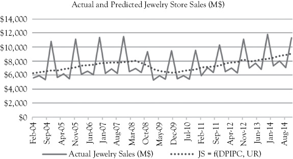
Figure 10.8 Jewelry sales as a function of disposable personal income per capita and the unemployment rate. The solid line represents actual sales while the dotted line is for the predicted values
The regression model for JS = f (DPIPC and UR) is shown in Figure 10.8. In this figure you see that by adding the unemployment rate the economic downturn in 2008 is more evident in the predicted values (the dotted line). What is missing is the seasonality in the actual jewelry sales.
Model 3. Jewelry Sales as a Function of Disposable Personal Income Per Capita (DPIPC), the Unemployment Rate (UR) and Seasonal Dummy Variables
In Figures 10.7 and 10.8 we saw that the two models used so far do not account for the seasonality in the jewelry sales data. This suggests that we might want to include dummy variables to account for the seasonality in the data. We know that we cannot use dummy variables for all four quarters. The most that we can use is three (one less than the number of possibilities for the seasonal aspect that we are trying to model).
We took the base model with jewelry sales as a function of DPIPC and UR and added dummy variables for quarters one, two, and three. The coefficients for the dummy variables representing all three quarters were negative which told us that quarter four was the highest quarter for jewelry sales. This was not a surprise since during the holiday season many people give jewelry as a gift. The quarter with the most negative coefficient was quarter three, indicating that Q3 is the lowest quarter for sales. We replaced Q3 with Q1 and found that the coefficient for Q1 had a P-value of about 0.30, indicating that Q1 is not significantly different than Q3. This told us that only Q2 and Q4 had significant seasonality.
Now we want a model with DPIPC, UR, Q2, and Q4. So we will now have the following model:
JS = f (DPIPC, UR, Q2, Q4).
The statistical results for this model are in Table 10.10.
Table 10.10 Jewelry sales (JS) as a function of disposable personal income per capita (DPIPC), the unemployment Rate (UR), and two dummy variables to account for seasonality
|
Jewelry sales = (DPIPC, UR, Q2, Q3) |
||||
|
Regression Statistics |
||||
|
R Square |
0.965 |
DW = 1.677 |
|
|
|
Adjusted R Square |
0.962 |
|
||
|
Standard Error |
400.765 |
|
||
|
Observations |
44 |
|
||
|
|
|
|||
|
|
Coefficients |
t Stat |
P-value |
P/2 |
|
Intercept |
956.111 |
1.328 |
0.192 |
0.096 |
|
DPIPC |
0.194 |
8.756 |
0.000 |
0.000 |
|
UR |
-262.435 |
-7.138 |
0.000 |
0.000 |
|
Q2 |
599.312 |
4.049 |
0.000 |
0.000 |
|
Q4 |
4,467.020 |
30.074 |
0.000 |
0.000 |
Step 1: Is the Model Logical?
One would still expect that jewelry sales would be positively related to how much money people have to spend. Therefore, the positive sign of the slope for DPIPC makes sense from an economic/business perspective. For the unemployment rate we might expect a negative relationship to jewelry sales because jewelry sales are generally something that could be delayed when consumers are worried about their employment situations. Thus, the negative coefficient for UR is logical. The positive coefficients for Q2 and Q4 are logical since the model is based on the lowest quarters of the year.
The regression equation is:
JS = 956.111 + 0.194(DPIPC) – 262.435(UR) + 599.312(Q2) + 4,467.020(Q4).
The actual JS data and the regression line for Model 3 are graphed in Figure 10.9. The dotted regression line in Figure 10.9 follows the actual values much better than either of the previous models.
Step 2: Are the Slope Terms Significantly Positive or Negative?
Once more the hypothesis for DPIPC is:
H0 : β ≤ 0
H1 : β > 0.
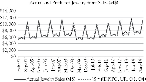
Figure 10.9 Jewelry sales as a function of disposable personal income per capita, the unemployment rate, and dummy variables for quarters two and four (Q2 and Q4). The solid line represents actual sales while the dotted line is for the predicted values
And, for the unemployment rate the hypothesis is:
H0 : β ≥ 0
H1 : β < 0.
For Q2 and Q3 the hypotheses would be:
H0 : β ≤ 0
H1 : β > 0.
Because the model is based on the lowest part of the year we expect the coefficients for other quarters to be positive.
To determine the t-table value, the degree of freedom (df) is still calculated as df = n – (k + 1). We know that n = 44 and now k = 4. Thus, df = 44 – (1 + 4) = 39. Again the t-table value is approximately 1.684 (see Appendix 4B, and use the row for df = 40, which is the closest value to 39).
The calculated t-ratio for disposable personal income is 8.756. This would far into the right tail of the distribution as indicated by a P-value of 0.000, and P/2 of 0.000. Notice that in this model the t-statistic for DPIPC is higher than either of the first two models. We see that the risk of error in rejecting the null hypothesis for DPIPC is low.
The calculated t-ratio for the unemployment rate is -7.138 which is more negative than the table value of –1.684. Again note that now that seasonality is accounted for the unemployment rate has a much higher t-statistic. Here both the P-value and P/2 are 0.000, which is far is less than 0.05.
For Q2 and Q4 the t-ratios are very large and positive. Thus, we have empirical support that there is a positive relationship between jewelry sales and quarters 2 and 4. The fourth quarter is high due to holiday gift giving. But, what about quarter 2? This quarter includes April, May, and June. These months include Mother’s Day, Father’s Day, many school graduations and many weddings. All of these can be occasions for which new jewelry might be purchased either for one’s self or as gifts.
Step 3: What is the Explanatory Power of the Model?
For this multiple regression model, the explanatory power is measured by the coefficient of determination, now the adjusted R2. In this model, the adjusted R2 is 0.962, which means 96.2 percent of the variation in jewelry store sales is explained by DPIPC, UR, Q2, and Q4. Now that seasonality is included the model is a great deal better than the first two models in terms of the explanatory power of the model.
Step 4: Check for Serial Correlation
The DW statistic for this model is 1.677. For this case, you would use dl = 1.285 and du = 1.721 with n = 40 and k = 4. Based on the table in Appendix 4C and the discussion in Appendix 4D you see that dl < 1.677 < 1.721, so Test 5 is again satisfied and therefore the result for this model is indeterminate with respect to serial correlation. Our calculated DW is close to du and all the t-statistics are quite large. Thus, we might not be too concerned about this result. Even if there is some upward bias in the t-statistics it is not likely to be enough to change our finding that there is a statistically significant relationship between jewelry sales and the four independent variables in the model.
Step 5: Check for Multicollinearity
Again we need to consider whether or not there may be multicollinearity. To check for this we look at the bivariate correlations between all pairs of independent variables. This is shown in Table 10.9. We see that there are no correlations that would be high enough to cause multicollinearity.
Observations
By reading the process of developing and evaluating these models for A&F sales and jewelry sales you will have solidified your understanding of multiple regression analysis. You will really learn about regression best by doing regression. You can start by entering the data from Table 3.1 for annual women’s clothing sales (WCS) into your own Excel file. Use the WCS data as your dependent variable and the year (time index) as your dependent variable. Then do the regression and verify that you get the same results as you saw in Chapter 3. After that, start to experiment with your own data.
What You Have Learned in Chapter 10
- You understand how to develop regression models
- You know how to apply the five step evaluation process to specific regression models.
- You understand how seasonal dummy variables can be selected so that all have positive coefficients and are statistically significant.
- You recognize how using seasonal dummy variables can sometimes greatly increase the explanatory power of a model.
1 We thank Laxmi Subhasini Rupesh for background research related to the A&F case.
2 SEC filings at www.sec.gov.
3 You would use 40 rather than n = 68 because the table only goes as high as 40.
4 For this case, you would use dl = 1.175 and du = 1.854.
