
Chapter 6: Creating Your First Pipeline
In Chapter 3, Pachyderm Pipeline Specification, we learned about the Pachyderm pipeline specification and what parameters you can configure in it. The pipeline specification is the most critical configuration piece of your pipeline, along with your code. In this chapter, we will learn how to create a Pachyderm pipeline that performs image processing. We will walk through all the steps that are involved in this process, including creating the Pachyderm repository, creating a pipeline, viewing the results of our computations, and adding an extra step to our original pipeline.
In this chapter, we will cover the following topics:
- Pipeline overview
- Creating a repository
- Creating a pipeline specification
- Viewing the pipeline result
- Adding another pipeline step
Technical requirements
This chapter requires that you have access to the following components and that they are installed and configured.
For a local macOS installation, you will need the following:
- macOS Mojave, Catalina, Big Sur, or later
- Docker Desktop for Mac 10.14
- minikube v1.19.0 or later
- pachctl 2.0.x or later
- Pachyderm 2.0.x or later
For a local Windows installation, you will need the following:
- Windows Pro 64-bit v10 or later
- Windows Subsystem for Linux (WSL) 2 or later
- Microsoft Powershell v6.2.1 or later
- Hyper-V
- minikube v1.19.0 or later
- kubectl v1.18 or later
- pachctl 2.0.x or later
- Pachyderm 2.0.x or later
For an Amazon Elastic Kubernetes Service (Amazon EKS) installation, you will need the following:
- kubectl v.18 or later
- eksctl
- aws-iam-authenticator
- pachctl 2.0.x or later
- Pachyderm 2.0.x or later
For a Microsoft Azure cloud installation, you will need the following:
- kubectl v.18 or later
- The Azure CLI
- pachctl 2.0.x or later
- Pachyderm 2.0.x or later
- jq 1.5 or later
For a Google Kubernetes Engine (GKE) cloud installation, you will need the following:
- Google Cloud SDK v124.0.0. or later
- kubectl v.18 or later
- pachctl 2.0.x or later
- Pachyderm 2.0.x or later
You do not need any special hardware to be able to run the pipelines in this chapter. If you are running your Pachyderm cluster locally, any modern laptop should support all the operations in this chapter. If you are running Pachyderm in a cloud platform, you will need to have a Persistent Volume (PV). See Chapter 5, Installing Pachyderm on a Cloud Platform, for more details.
All the scripts and data described in this chapter are available at https://github.com/PacktPublishing/Reproducible-Data-Science-with-Pachyderm/tree/main/Chapter06-Creating-Your-First-Pipeline.
Now that we have reviewed the technical requirements for this chapter, let's take a closer look at our pipeline.
Pipeline overview
In Chapter 4, Installing Pachyderm Locally, and Chapter 5, Installing Pachyderm on a Cloud Platform, we learned how to deploy Pachyderm locally or on a cloud platform. By now, you should have some version of Pachyderm up and running, either on your computer or a cloud platform. Now, let's create our first pipeline.
A Pachyderm pipeline is a technique that processes data from a Pachyderm input repository or repositories and uploads it to a Pachyderm output repository. Every time new data is uploaded to the input repository, the pipeline automatically processes it. Every time new data lands in the repository, it is recorded as a commit hash and can be accessed, rerun, or analyzed later. Therefore, a pipeline is an essential component of the Pachyderm ecosystem that ensures the reproducibility of your data science workloads.
To get you started quickly, we have prepared a simple example of image processing that will draw a contour on an image. A contour is an outline that represents the shape of an object. This is a useful technique that is often applied to image processing pipelines.
Image processing is a widely used technique that enables you to enhance the quality of images, transform an image into another image, extract various information about an image, and so on. With machine learning, you can set up pipelines that can determine objects in an image, create a histogram of an image, and so on.
There are many open source libraries that you can use for advanced image processing, with the most famous among them being OpenCV and scikit-image. Both of these libraries are widely used by machine learning experts for various image processing tasks.
For this example, we will use scikit-image. Scikit-image, or skimage, is an open-source image processing library that enables you to run various image processing algorithms to analyze and transform images. Scikit-image is built to work with the Python programming language.
In this example, we will use scikit-image with a couple of other open source components, including the following:
- NumPy: An open source Python library that enables you to work with arrays. When you need to analyze or segment an image, it must be transformed into an array for processing.
- Matplotlib: An extension to NumPy that enables you to plot images and create data visualizations.
We will create a pipeline that will consume the data from the photos repository, run a contour.py script against the images in the photos repository, and upload the result to the contour output repository.
The following diagram explains our pipeline:
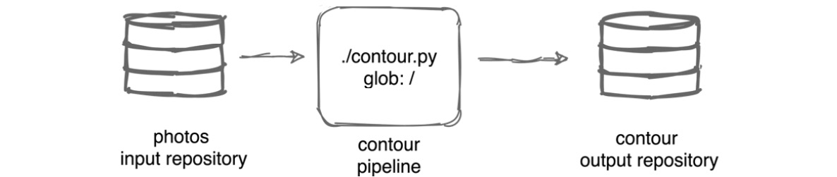
Figure 6.1 – Contour pipeline
The following code explains the contour.py script:
import numpy as np
import matplotlib.pyplot as plt
import os
from skimage.io import imread, imsave
from skimage import measure
import logging
logging.basicConfig(level=logging.INFO)
def create_contours(photo):
image = imread(photo, as_gray=True)
t = os.path.split(photo)[1]
c = measure.find_contours(image, 0.9)
fig, ax = plt.subplots()
ax.imshow(image, vmin=-1, vmax=1, cmap='gray')
for contour in c:
ax.plot(contour[:, 1], contour[:, 0], linewidth=2)
ax.axis('image')
ax.set_xticks([])
ax.set_yticks([])
plt.savefig(os.path.join("/pfs/out", os.path.splitext(t)[0]+'.png'))
for dirpath, dirnames, filenames in os.walk("/pfs/photos"):
for f in filenames:
create_contours(os.path.join(dirpath, f))
The preceding script contains a function called create_contours. This function does the following:
- First, it reads the image file from the pfs/photos repository and converts it into a grayscale image. This is needed to transform a color image (RGB) into a two-dimensional NumPy array.
- Then, it uses the measure.find_contours API method from the skimage.measure.find_contours module to find the contour of the two-dimensional array that we converted our image into at a value of 0.9. This value represents the position between light and dark tones. Typically, it's best to use a middle value, but in this case, 0.9 created the best results.
- Then, it defined subplots to visualize our image and saved it in the pfs/out directory, which, in reality, will be the pfs/out/contour output repository.
- The last part of the script tells the program to apply the create_contours function to all the files in the pfs/photos repository.
This script is built into a Docker image that we will use to run our pipeline. This Docker image is hosted in Docker Hub.
We will use the following images from freepik.com for processing. The first image is an image of a brown vase:

Figure 6.2 – Brown vase
The second image is an image of a hand:

Figure 6.3 – Hand
Finally, the third image is an image of a landscape:

Figure 6.4 – Landscape
As you can see, these are some simple images where finding the contours should be easy. You can try to run this pipeline against more complex images and see the results you'll get. In general, the more contrast you have between the elements in the image, the more precise contours the algorithm will be able to find.
Now that we understand the example we are working on, let's go ahead and create a repository.
Creating a repository
The first step in creating your pipeline is to create a Pachyderm repository and put some data in it. As you probably remember from Chapter 2, Pachyderm Basics, a Pachyderm repository is a location inside of a Pachyderm cluster where you store your data. We will be creating an input repository, and the pipeline will automatically create an output repository on the first run.
To create an input repository, perform the following steps:
- Log into your Terminal.
- Verify that Pachyderm is up and running:
% pachctl version
You should see an output similar to the following:
COMPONENT VERSION
pachctl 2.0.0
pachd 2.0.0
The pachd component must list a version.
- Create a Pachyderm input repository called photos:
% pachctl create repo photos
No output will be returned.
You should see the following output:
NAME CREATED SIZE (MASTER) ACCESS LEVEL
photos 11 seconds ago ≤ 0B [repoOwner]
Here, you can see that the photos repository was created and that it is empty. Although the size is counted for the master branch, at this point, no branches exist in this repository. Pachyderm will automatically create a specified branch when you put files in it.
- Put some images in the photos repository. We need to put the files into the root of our photos repository. To do this, you need to use the -r (recursive) flag and specify the path to the directory that contains the files on your computer. For example, if you have downloaded the files to a data folder on your computer, you need to run the following command:
% pachctl put file -r photos@master:/ -f data
The following is some sample output:
data/brown_vase.png 25.82 KB / 25.82 KB [=====] 0s 0.00 b/s
data/hand.png 33.21 KB / 33.21 KB [======] 0s 0.00 b/s
data/landscape.png 54.01 KB / 54.01 KB [=========] 0s
Pachyderm automatically creates the specified branch. In this example, Pachyderm creates the master branch. You could name the branch anything you want, but for simplicity, let's call it master. All the commands in this section are written with the master branch in mind.
The following is some sample output:
NAME TYPE SIZE
/brown_vase.png file 25.21KiB
/hand.png file 32.43KiB
/landscape.png file 52.74KiB
- Alternatively, you could place each file one by one by running the pachctl put file command for each image. For example, to place the landscape.jpg file, change the directory on your computer to data and use the following command:
% pachctl put file photos@master -f landscape.jpg
The following is some sample output:
data/landscape.jpg 54.01KB / 54.01 KB [=] 0s 0.00 b/s/
Repeat this command for all image files.
Important note
Make sure that the TYPE parameter in the output says file and not dir. Pachyderm does not distinguish between directories and files, and you use -f to put files in a directory or the root of the repository. If any of your files are listed as dir, you need to delete them by running pachctl delete file photos@master:<path> and start over. The pipeline will not work as expected if you place the files in the directories.
Now that we have created a repository, let's create our pipeline specification.
Creating a pipeline specification
In the Creating a repository section, we created a repository called photos and put some test files in it. The pipeline specification for this example must reference the following elements:
- An input repository with data to process
- A computer program or a script that needs to run against your data
- A glob pattern that specifies the datum granularity
- A Docker image with built-in dependencies that contains your code
We have created a pipeline specification for you so that you can use it to create the pipeline. Here is what is in the pipeline specification file in the YAML Ain't Markup Language (YAML) format:
---
pipeline:
name: contour
description: A pipeline that identifies contours on an image.
transform:
cmd:
- python3
- "/contour.py"
image: svekars/contour-histogram:1.0
input:
pfs:
repo: photos
glob: "/"
Let's look at the pipeline specification in more detail. Here are the parameters in the pipeline:

Figure 6.5 – Contour pipeline parameters
This pipeline specification does not include any optimization or other extra parameters. It is a minimum pipeline that will do the required computation for our example.
To create a pipeline, perform the following steps:
- Log into your terminal.
- Create the contour pipeline by running the following command:
% pachctl create pipeline -f contour.yaml
No output will be returned.
- Verify that the pipeline has been created:
% pachctl list pipeline
The following is the system output:
NAME VERSION INPUT CREATED STATE / LAST JOB DESC
contour 1 photos:/* 5 seconds ago running / - A pipeline that identifies contours on an image.
As soon as you create the pipeline, it will set its status to running and attempt to process the data in the input repository. You might also see that LAST JOB is set to starting or running.
Important note
Another important thing in the preceding output is the pipeline version. The version of our pipeline is 1. If you change anything in your pipeline's YAML file and update your pipeline after that, the version counter will be updated to a subsequent number.
- View the job that has been started for your pipeline:
pachctl list job
The following is the system output:
ID SUBJOBS PROGRESS CREATED MODIFIED
71169d… 1 2 minutes ago 2 minutes ago
The output of the pachctl list job command gives us the following information:

Figure 6.6 – Pipeline output explained
Now that our pipeline has run successfully, let's see the output in the output repository.
Viewing the pipeline result
Once your pipeline has finished running, you can view the result in the output repository. We will look at the output result in both the command line and the Pachyderm dashboard for visibility.
If you are using a local Pachyderm deployment with minikube, you need to enable port-forwarding before you can access the Pachyderm UI.
To view the pipeline result in the terminal, perform the following steps:
- Log into your terminal.
- Verify that the output repository called contour has been created:
% pachctl list repo
The following is the system output:
% pachctl list repo
NAME CREATED SIZE (MASTER) ACCESS LEVEL
contour About a minute ago ≤ 117.6KiB [repoOwner] Output repo for pipeline contour.
photos 5 minutes ago ≤ 110.4KiB [repoOwner] B
As you can see, the contour repository has been created, and it contains 117.6 KiB of data. If you are running Pachyderm locally, you can also preview what those files look like by running one of the following commands.
- If you are on macOS, run the following command to list the files in the output repository:
% pachctl list file contour@master
The following is the system output:
NAME TYPE SIZE
/brown_vase.png file 23.78KiB
/hand.png file 29.79KiB
/landscape.png file 64.08Kib
- Now, pipe the open command to the pachctl get file command to open one of the images in the default preview application on your Mac. For example, to preview hand.png, run the following command:
% pachctl get file contour@master:hand.png | open -f -a Preview.app
You should see the following output:

Figure 6.7 – Hand processed
Now, let's view the processed results in the UI. If you are running Pachyderm on a cloud provider, just point your browser to the IP address where the Pachyderm dashboard is running. If you are running Pachyderm in Pachyderm Hub, follow the instructions in Pachyderm Hub to access the console. If you are running Pachyderm locally in minikube, follow the remaining steps to enable port-forwarding.
Important note
Unless you are running your experiments in Pachyderm Hub, the Pachyderm console is only available if you have deployed it. You need to have a trial or an enterprise license to deploy the Pachyderm console locally or in the cloud.
- Open a separate terminal window.
- Enable port forwarding for your local Pachyderm deployment by running the following command:
% pachctl port-forward
You should see the following output:
Forwarding the pachd (Pachyderm daemon) port...
listening on port 30650
Forwarding the pachd (Pachyderm daemon) port...
listening on port 30650
Forwarding the OIDC callback port...
listening on port 30657
Forwarding the s3gateway port...
listening on port 30600
Forwarding the identity service port...
listening on port 30658
Forwarding the dash service port...
...
If you have used the default settings, the Pachyderm dashboard must load at http://localhost:30080.
- Paste the dashboard IP address into a web browser.
- If you are prompted to log in, follow the onscreen instructions to do so. When you log in, you should see the following screen:

Figure 6.8 – Pachyderm Direct Acyclic Graph (DAG)
This is a Direct Acyclic Graph (DAG) that's been created for the input and output repositories, as well as the pipeline.
- Click on the contour output repository (the last one on the screen) and then click View Files:

Figure 6.9 – Output repository information
- Click Preview next to hand.png:
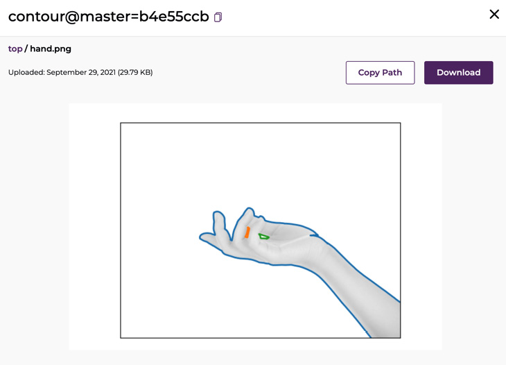
Figure 6.10 – Output file
You can preview all the resulting files from the UI in the same way. From here, the files can be either consumed by another pipeline or served outside of Pachyderm through an S3 Gateway, or the output repository can be mounted and accessible on a local disk. Let's look at what the other images should look like.
You should see that the landscape image has changed, as follows:

Figure 6.11 – Processed landscape image
The brown_vase.png image should look like this:
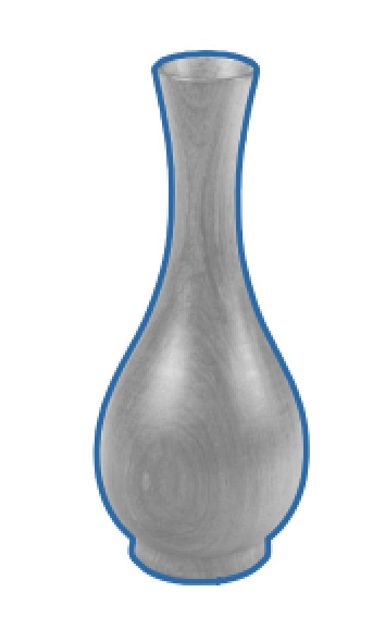
Figure 6.12 – Processed vase image
In this section, we learned how to view the results of a pipeline. Now, let's add another pipeline step.
Adding another pipeline step
Pachyderm pipelines can be chained into multi-step workflows. For each step, you will need to have a separate pipeline specification and a Docker image if you are using one. In this section, we will add another step to our image processing workflow. We will use the skimage.exposure.histogram module to create histograms of all the images we have in our contour output repository.
Example overview
A histogram is a visual representation of data that provides information about the image, such as the number of pixels, their intensity, and other information. Because we represent images as numerical data, we can create a histogram for each of the images we processed in the first step of our workflow – the contour pipeline. In this new step of the workflow, we will create histograms for each image that has landed in the contour output repository and save them in the histogram output repository in PNG format.
Here is an example of a histogram that has been generated for the hand.png image:

Figure 6.13 – Grayscale image histogram
The y-axis represents the count of pixels, while the x-axis represents the intensity of the pixels.
Here is a diagram of the new two-step workflow, which includes the contour and histogram pipelines:

Figure 6.14 – Contour and histogram workflow
The histogram pipeline will consume the files from the contour repository, create histograms for them, and output them to the histogram repository.
Histogram creation script overview
In this pipeline step, we will use histogram.yaml, which will create a pipeline for us. The pipeline will run the histogram.py script.
Let' review the histogram.py script, which creates histograms from the file in the contour repository:
from skimage import io
import matplotlib.pyplot as plt
import numpy as np
import os
def create_histogram(photo):
image = io.imread(photo)
t = os.path.split(photo)[1]
plt.hist(image.ravel(), bins=np.arange(10, 70), color='blue', alpha=0.5, rwidth=0.7)
plt.yscale('log')
plt.margins(x=0.03, y=-0.05)
plt.xlabel('Intensity')
plt.ylabel('Count')
plt.savefig(os.path.join("/pfs/out", os.path.splitext(t)[0]+'.png'))
for dirpath, dirnames, filenames in os.walk("/pfs/contour"):
for f in filenames:
create_histogram(os.path.join(dirpath, f))
This script imports the following libraries:
- skimage.io: The io module from the scikit-image library enables read and write operations within your Python file. We need this module to read files from the contour repository.
- matploit.pyplot: This Matplotlib interface enables us to plot our images. We use it to create the histogram, add labels to the x- and y-axis of the plot, and so on.
- numpy: We need NumPy to represent the image as an array and keep the number of bins in the required range.
- os: The os module from the standard Python library enables read and write operations with files. We need this module to read images from the Pachyderm contour repository and save our images in the correct output repository.
Let's take a closer look at what the script does. The create_histogram function reads image files from the contour repository. Then, using the matploit.pyplot.hist (plt.hist) function, the script creates a histogram with the following parameters:
- The numpy.ravel function converts our images from the 2D array into a 1D array, which is needed to plot a histogram.
- The bins parameter defines the shape and distribution of vertical bars in your histogram. To distribute them evenly on the plot, we have a defined range by using the np.arange function.
- The color='blue' parameter defines the color of the histogram bins.
- The alpha=0.5 parameter defines the level of transparency.
- The rwidth=0.7 parameter defines the width of each bin.
- The plt.yscale('log') parameter defines the logarithmic y-axis scale. We need this parameter to narrow the scale of the y-axis for better data visualization.
- The plt.margins(x=0.03, y=-0.05) parameter determines the amount of whitespace between the histogram and the start of the plot.
- The plt.xlabel('Intensity') and plt.ylabel('Count') parameters define the labels for the x- and y-axes.
- The plt.savefig function defines where to save the histogram. In our case, we will save it in the pfs/out directory, in which Pachyderm will automatically create a histogram repository under the pfs/out/histogram path.
Important note
In your scripts, you do not need to add the path to the repository, just to the pfs/out directory.
Pipeline specification overview
The histogram.yaml pipeline specification creates the histogram pipeline.
Here is what our pipeline specification will look like:
---
pipeline:
name: histogram
description: A pipeline that creates histograms for images stored in the contour repository.
transform:
cmd:
- python3
- "/histogram.py"
image: svekars/contour-histogram:1.0
input:
pfs:
repo: contour
glob: "/"
This pipeline does the following:
- Uploads the files stored in the contour repository as a single datum
- Pulls the Docker image stored in Docker Hub under svekars/histogram:1.0
- Runs the histogram.py script against all the files that have been downloaded from the contour repository
- Uploads the results of the transformation to the histogram output repository
Now that we have reviewed what goes into this pipeline, let's go ahead and create it.
Creating the pipeline
The next step is to create the histogram pipeline, which will create a histogram for each image in the photos repository.
Let's create the second step of our workflow by using the histogram.yaml file:
- Log into your terminal.
- Verify that Pachyderm is up and running:
% pachctl version
The following is the system output:
COMPONENT VERSION
pachctl 2.0.0
pachd 2.0.0
If pachd is unresponsive, you might need to run minikube stop and minikube start in a local installation to be able to resume working with it. If you are in a cloud environment, you will need to check your connection. If you are running Pachyderm in Pachyderm Hub, check that you are authenticated from the console and follow the onscreen instructions.
- Create the histogram pipeline:
% pachctl create pipeline -f histogram.yaml
No system output will be returned.
- Verify that the pipeline was created:
% pachctl list pipeline
The following is the system output:
NAME VERSION INPUT CREATED STATE / LAST JOB DESCRIPTION
contour 1 photos:/* 12 minutes ago running / success A pipeline that identifies contours on an image.
histogram 1 contour:/ 12 seconds ago running / success A pipeline that creates histograms for images stored in the contour repository.
According to the preceding output, the histogram pipeline was created and is currently running the code.
The following is the system output:
NAME CREATED SIZE (MASTER) DESCRIPTION
histogram 23 seconds ago ≤ 27.48KiB [repoOwner] Output repo for pipeline histogram.
contour 24 minutes ago ≤ 117.6KiB [repoOwner] Output repo for pipeline contour.
photos 29 minutes ago ≤ 110.4KiB [repoOwner]
The histogram output repository was created and contains 27.48 KiB of data. These are our histogram files.
- List the files in the histogram repository:
% pachctl list file histogram@master
The following is the system output:
NAME TYPE SIZE
/hand.png file 9.361KiB
/landscape.png file 9.588KiB
/brown_vase.png file 8.526KiB
With that, our histogram visualizations have been added to the repository.
- View the histogram files. For example, if you are on Mac, to view the landscape.png histogram file, run the following command:
pachctl get file histogram@master:landscape.png | open -f -a Preview.app
Here is the resulting histogram:

Figure 6.15 – Histogram of the landscape image
You can preview other files in a similar way or through the Pachyderm dashboard, as described earlier.
- Go to the console and view the DAG for this newly added pipeline:

Figure 6.16 – Updated DAG
As you can see, you now have a new pipeline called histogram and a new eponymous output repository added to your DAG.
Now that we have created our first pipeline, let's clean up our environment so that we have a clean cluster to work on the tasks in the next chapter.
Cleaning up
Once you are done experimenting, you might want to clean up your cluster so that you start your next experiment with a fresh install. To clean up the environment, perform the following steps:
- Delete all the pipelines and repositories:
pachctl delete pipeline –all && pachctl delete repo --all
- Verify that no repositories and pipelines exist in your cluster:
pachctl list repo && pachctl list pipeline
You should see the following output:
NAME CREATED SIZE (MASTER) DESCRIPTION
NAME VERSION INPUT CREATED STATE / LAST JOB DESCRIPTION
With that, you have successfully cleaned up your cluster.
Summary
In this chapter, you successfully created your first Pachyderm repository, pipeline, and even extended it with another pipeline step. We used scikit-image, Matplotlib, and NumPy to create contours on images stored in Pachyderm repositories and created histograms for all of these images. This is the first step in understanding how Pachyderm works. In Pachyderm, you'll work with pipelines quite a lot. As you have already noticed, you can put any code in your pipeline. Although most of the examples in this book will use Python, you can use any programming language of your choice.
In the next chapter, we will learn more about Pachyderm functionality, how to ingest data into Pachyderm and export it to outside systems, how to make changes to a pipeline's code, how to tune various parameters, and other important Pachyderm operations.
Further reading
For more information about the topics that were covered in this chapter, take a look at the following resources:
- Docker Hub documentation: https://docs.docker.com/docker-hub/
- Matplotlib documentation: https://matplotlib.org/
- NumPy documentation: https://numpy.org/doc/stable/
- Scikit-image documentation: https://scikit-image.org
- Landscape image: https://www.freepik.com/free-vector/beautiful-gradient-spring-landscape_6969720.htm
- Brown vase image: https://www.freepik.com/free-photo/narrow-neck-vase_921733.htm
- Hand image: https://www.freepik.com/free-photo/hand-holding-something-with-white-background_978615.htm