Chapter 9: Modeling Categorical Variables
Gradient Boosting, Forests, and Neural Networks
In Chapter 8, we introduced linear regressions, generalized linear models and regression trees for modeling continuous response variables. In this chapter, we focus on applications in which the response variable is categorical, such as organic food that is purchased in a supermarket (Bought, Not), blood press status (High, Normal, Low), and credit card application status (Accepted, Rejected). Logistic regressions and decision trees are introduced in the first two sections for a binary response variable, which is a response variable with only two qualitative outcomes. In the last section, we introduce random forests, gradient boosting trees, and neural networks, which can fit a categorical response variable with more than two distinct outcomes.
We continue to use the Organics data set for this chapter. Again, we assume that a CAS server is already set up and the data sets have been loaded to the CAS server
In [1]: organics.tableinfo()
Out[1]:
[TableInfo]
Name Rows Columns Encoding CreateTimeFormatted
0 ORGANICS 1688948 36 utf-8 09Nov2016:10:32:06
ModTimeFormatted JavaCharSet CreateTime ModTime
0 09Nov2016:10:32:06 UTF8 1.794307e+09 1.794307e+09
Global Repeated View SourceName SourceCaslib Compressed
0 1 0 0 0
Creator Modifier
0 username
Logistic Regression
Similar to the linear regression models introduced in Chapter 8, logistic regression uses the linear combination of one or more predictors to build a predictive model for the response outcomes. Unlike linear regressions, the prediction of interest in a logistic regression is not a continuous outcome with a range from negative to positive infinity. Instead, we are interested in predicting the probabilities of the outcome levels of the response variable. Examples are the probability of buying or not buying organic food from a supermarket or the probability of a credit card application that is accepted or rejected. For a binary response variable, the two distinct outcome levels are usually called the event level and the non-event level.
We simply need to predict Pevent, the event probability for the response variable, which always takes values in [0, 1]. Logistic regression originates from the logistic transformation, which maps a continuous input from (−∞, ∞) to an output between 0 and 1.

Similarly, a logistic regression model uses the logistic transformation to link the linear combination of one or more predictors to the probability of event level as follows:
where t is a linear combination of the predictors:
The inverse form of the transformation also indicates that a logistic regression is a non-linear model:
where the function G(Pevent) is often called the logit link function. The ratio Pevent/1 − Pevent) is also known as the odds ratio. When a logit link function is used, we assume that the predictors have a linear relationship with the log of the odds ratio. Logistic regression can be extended by using other link functions as well, such as probit, cloglog, and negative cloglog.
Logistic regression models are available in the regression action set. First, you must load the action set.
In [2]: conn.loadactionset('regression')
Now let’s build a simple logistic regression for the Organics data to predict whether consumers would like to buy organic food. The response variable in this data is called TargetBuy.
In [2]: organics.logistic(
...: target = 'TargetBuy',
...: inputs = ['DemAge', 'Purchase_3mon', 'Purchase_6mon']
...: )
NOTE: Convergence criterion (GCONV=1E-8) satisfied.
Out[2]:
[ModelInfo]
Model Information
RowId Description Value
0 DATA Data Source ORGANICS
1 RESPONSEVAR Response Variable TargetBuy
2 DIST Distribution Binary
3 LINK Link Function Logit
4 TECH Optimization Technique Newton-Raphson with Ridging
[NObs]
Number of Observations
RowId Description Value
0 NREAD Number of Observations Read 1688948.0
1 NUSED Number of Observations Used 1574340.0
[ResponseProfile]
Response Profile
OrderedValue Outcome TargetBuy Freq Modeled
0 1 Bought Bought 387600.0 *
1 2 No No 1186740.0
[ConvergenceStatus]
Convergence Status
Reason Status MaxGradient
0 Convergence criterion (GCONV=1E-8) s... 0 4.419888e-08
[Dimensions]
Dimensions
RowId Description Value
0 NDESIGNCOLS Columns in Design 4
1 NEFFECTS Number of Effects 4
2 MAXEFCOLS Max Effect Columns 1
3 DESIGNRANK Rank of Design 4
4 OPTPARM Parameters in Optimization 4
[GlobalTest]
Testing Global Null Hypothesis: BETA=0
Test DF ChiSq ProbChiSq
0 Likelihood Ratio 3 149251.090674 0.0
[FitStatistics]
Fit Statistics
RowId Description Value
0 M2LL -2 Log Likelihood 1.608090e+06
1 AIC AIC (smaller is better) 1.608098e+06
2 AICC AICC (smaller is better) 1.608098e+06
3 SBC SBC (smaller is better) 1.608147e+06
[ParameterEstimates]
Parameter Estimates
Effect Parameter ParmName DF Estimate
0 Intercept Intercept Intercept 1 1.755274
1 DemAge DemAge DemAge 1 -0.057438
2 purchase_3mon purchase_3mon purchase_3mon 1 -0.000002
3 purchase_6mon purchase_6mon purchase_6mon 1 0.000039
StdErr ChiSq ProbChiSq
0 0.057092 945.232627 1.442299e-207
1 0.000158 131358.158671 0.000000e+00
2 0.000055 0.000866 9.765250e-01
3 0.000039 0.990883 3.195267e-01
[Timing]
Task Timing
RowId Task Time RelTime
0 SETUP Setup and Parsing 0.017694 0.058605
1 LEVELIZATION Levelization 0.027966 0.092627
2 INITIALIZATION Model Initialization 0.000611 0.002024
3 SSCP SSCP Computation 0.017766 0.058843
4 FITTING Model Fitting 0.233353 0.772892
5 CLEANUP Cleanup 0.002567 0.008502
6 TOTAL Total 0.301922 1.000000
In the preceding example, we build a logistic regression to predict the probability of buying organic food (Pr(TargetBuy = Bought)) using three continuous predictors Age, Recent 3 Month Purchase Amount, and Recent 6 month Purchase Amount. You can also add categorical predictors to the logistic regression. They must be specified in both the inputs argument and the nominals argument.
In [3]: organics.logistic(
...: target = 'TargetBuy',
...: inputs = ['DemAge', 'Purchase_3mon', 'Purchase_6mon', 'DemGender',
'DemHomeowner'],
...: nominals = ['DemGender', 'DemHomeowner'],
...: display = {'names': ['ParameterEstimates']}
...: )
NOTE: Convergence criterion (GCONV=1E-8) satisfied.
Out[3]:
[ParameterEstimates]
Parameter Estimates
Effect DemGender DemHomeowner Parameter
0 Intercept Intercept
1 DemAge DemAge
2 purchase_3mon purchase_3mon
3 purchase_6mon purchase_6mon
4 DemGender F DemGender F
5 DemGender M DemGender M
6 DemGender U DemGender U
7 DemHomeowner No DemHomeowner No
8 DemHomeowner Yes DemHomeowner Yes
ParmName DF Estimate StdErr ChiSq
0 Intercept 1 0.353349 0.059586 35.165819
1 DemAge 1 -0.056478 0.000162 120824.157416
2 purchase_3mon 1 0.000009 0.000057 0.024229
3 purchase_6mon 1 0.000037 0.000040 0.819283
4 DemGender_F 1 1.817158 0.007381 60608.910532
5 DemGender_M 1 0.857905 0.008216 10904.528993
6 DemGender_U 0 0.000000 NaN NaN
7 DemHomeowner_No 1 0.000320 0.004226 0.005725
8 DemHomeowner_Yes 0 0.000000 NaN NaN
ProbChiSq
0 3.027918e-09
1 0.000000e+00
2 8.763032e-01
3 3.653900e-01
4 0.000000e+00
5 0.000000e+00
6 NaN
7 9.396871e-01
8 NaN
In the preceding example, we also use the display option to select only the parameter estimate output table. For each categorical predictor, the logistic action constructs dummy indicators for the distinct levels of the predictor, and uses them as linear terms. For example, if a consumer is 30 years old, has purchased the amount $1,200 and $500 for the last six months and three months, respectively, is male, and currently does not own a home, the predicted probability of buying organic food is 39.65%.
t=0.3533−0.056×30+0.000008864×500+0.00003651×1200+0.8579+0.0003197=−0.42024
The following table summarizes the output tables that are returned by the logistic action.
| Table Name | Description |
| NObs | The number of observations that are read and used. Missing values are excluded, by default. |
| ResponseProfile | The frequency distribution of the response variable. The event level is marked with an asterisk (*). |
| ConvergenceStatus | The convergence status of the parameter estimation. |
| Dimension | The dimension of the model, including the number of effects and the number of parameters. |
| GlobalTest | A likelihood ratio test that measures the overall model fitting. |
| FitStatistics | The fit statistics of the model such as log likelihood (multiplied by -2), AIC, AICC and BIC. |
| ParameterEstimates | The estimation of the logistic regression parameters. |
| Timing | A timing of the subtasks of the GLM action call. |
In Python, you can define the logistic model first and add options, step-by-step, which enables you to reuse a lot of code when you need to change only a few options in a logistic model. The preceding logistic action code can be rewritten as follows:
In [4]: all_preds = ['DemAge', 'Purchase_3mon', 'Purchase_9mon', 'DemGender',
'DemHomeowner']
...: all_cats = ['DemGender', 'DemHomeowner']
...:
...: model1 = organics.Logistic()
...: model1.nominals = all_cats
...: model1.target = 'TargetBuy'
...: model1.inputs = all_preds
...: model1.display.names = ['ParameterEstimates']
...:
...: model1()
In the preceding example, first, we define a new logistic model model1, and then add the class effect list (model1.nominals), the response variables (model1.target), and the effect list (model1.inputs), step-by-step. The logistic action, by default, uses the logit link function but you can always override it with your own event selection. In the following example, we reuse the model1 definition from the previous example and change the link function to PROBIT:
In [5]: model1.link = 'PROBIT'
...: model1.display.names = ['ResponseProfile', 'ParameterEstimates']
...: model1()
NOTE: Convergence criterion (GCONV=1E-8) satisfied.
Out[5]:
[ResponseProfile]
Response Profile
OrderedValue Outcome TargetBuy Freq Modeled
0 1 Bought Bought 387600.0 *
1 2 No No 1186740.0
[ParameterEstimates]
Parameter Estimates
Effect DemGender DemHomeowner Parameter
0 Intercept Intercept
1 DemAge DemAge
2 purchase_3mon purchase_3mon
3 purchase_9mon purchase_9mon
4 DemGender F DemGender F
5 DemGender M DemGender M
6 DemGender U DemGender U
7 DemHomeowner No DemHomeowner No
8 DemHomeowner Yes DemHomeowner Yes
ParmName DF Estimate StdErr ChiSq
0 Intercept 1 0.447991 0.072359 38.330834
1 DemAge 1 -0.056478 0.000162 120823.996353
2 purchase_3mon 1 0.000071 0.000049 2.074100
3 purchase_9mon 1 -0.000026 0.000029 0.811013
4 DemGender_F 1 1.817162 0.007381 60609.158117
5 DemGender_M 1 0.857905 0.008216 10904.528278
6 DemGender_U 0 0.000000 NaN NaN
7 DemHomeowner_No 1 0.000318 0.004226 0.005669
8 DemHomeowner_Yes 0 0.000000 NaN NaN
ProbChiSq
0 5.971168e-10
1 0.000000e+00
2 1.498183e-01
3 3.678210e-01
4 0.000000e+00
5 0.000000e+00
6 NaN
7 9.399814e-01
8 NaN
The logistic regression models that we have built so far train the model without actually using the model to make a prediction (that is, estimating P(event)). You must specify an output table for the logistic action in order to score the observations in the input table. By default, the casout table contains only the predictions, but you can use the copyvars option to copy some columns from the input table to the casout table. You can use copyvars=’all’ to copy all columns to the casout table.
In [6]: result1 = conn.CASTable('predicted', replace=True)
...: model1.output.casout = result1
...: model1.output.copyvars = 'all'
...: del model1.display
...: model1()
The logistic action generates one more result tables when a casout table is created. This table contains basic information about the casout table such as the name, the library, and the dimensions of the table.
[OutputCasTables]
casLib Name Label Rows Columns
0 CASUSERHDFS(username) predicted 1688948 37
casTable
0 CASTable('predicted', caslib='CASUSE...
You can print out the column names of the output table to see what new columns have been added. By default, the logistic action creates a new column _PRED_ for the estimated event probability.
In [7]: result1.columns
Out[7]:
Index(['_PRED_', 'ID', 'DemAffl', 'DemAge', 'DemGender',
'DemHomeowner', 'DemAgeGroup', 'DemCluster', 'DemReg',
'DemTVReg', 'DemFlag1', 'DemFlag2', 'DemFlag3', 'DemFlag4',
'DemFlag5', 'DemFlag6', 'DemFlag7', 'DemFlag8', 'PromClass',
'PromTime', 'TargetBuy', 'Bought_Beverages', 'Bought_Bakery',
'Bought_Canned', 'Bought_Dairy', 'Bought_Baking',
'Bought_Frozen', 'Bought_Meat', 'Bought_Fruits',
'Bought_Vegetables', 'Bought_Cleaners', 'Bought_PaperGoods',
'Bought_Others', 'purchase_3mon', 'purchase_6mon',
'purchase_9mon', 'purchase_12mon'],
dtype='object')
You can use the data summary actions in the simple action set to look at the model output. For example, let’s compare the average predicted probability of buying organic foods across different levels of DemGender:
In [8]: result1.crosstab(row='DemGender', weight='_PRED_', aggregators='mean')
Out[8]:
[Crosstab]
DemGender Col1
0 F 0.343891
1 M 0.165559
2 U 0.076981
From the preceding output, it looks like female customers are more likely to purchase organic food, and the customers who didn’t provide gender information are not interested in buying organic food. The ratio (0.343891/0.076981) between these two groups is approximately 5, which means female customers are five times more likely to purchase organic foods than the customers who didn’t provide gender information.
The logistic action generates additional model diagnosis outputs. The following table summarizes the columns that a logistic action can generate as output.
| Option | Description |
| pred | The predicted value. If you do not specify any output statistics, the predicted value is named _PRED_, by default. |
| resraw | The raw residual. |
| xbeta | The linear predictor. |
| stdxbeta | The standard error of the linear predictor. |
| lcl | The lower bound of a confidence interval for the linear predictor. |
| ucl | The upper bound of a confidence interval for the linear predictor. |
| lclm | The lower bound of a confidence interval for the mean. |
| uclm | The upper bound of a confidence interval for the mean. |
| h | The leverage of the observation. |
| reschi | The Pearson chi-square residual. |
| stdreschi | The standardized Pearson chi-square residual. |
| resdev | The deviance residual. |
| reslik | The likelihood residual (likelihood displacement). |
| reswork | The working residual. |
| difdev | The change in the deviance that is attributable to deleting the individual observation. |
| difchisq | The change in the Pearson chi-square statistic that is attributable to deleting the individual observation. |
| cbar | The confidence interval displacement, which measures the overall change in the global regression estimates due to deleting the individual observation. |
| alpha | The significance level used for the construction of confidence intervals. |
Similar to the code argument in the glm action for linear regression, SAS DATA step code can also be used to save a logistic model. You can score new data sets using the DATA step code in Python (using the runcode action from the datastep action set) or in a SAS language environment such as Base SAS or SAS Studio.
In [9]: # example 4 score code
...: result = organics.logistic(
...: target = 'TargetBuy',
...: inputs = ['DemAge', 'Purchase_3mon', 'Purchase_6mon'],
...: code = {}
...: )
NOTE: Convergence criterion (GCONV=1E-8) satisfied.
In [10]: result['_code_']
Out[10]:
Score Code
SASCode
0 /*-------------------------------...
1 Generated SAS Scoring Code
2 Date: 09Nov2016:13:33:15
3 -------------------------------...
4
5 drop _badval_ _linp_ _temp_ _i_ _j_;
6 _badval_ = 0;
7 _linp_ = 0;
8 _temp_ = 0;
9 _i_ = 0;
10 _j_ = 0;
11
12 array _xrow_0_0_{4} _temporary_;
13 array _beta_0_0_{4} _temporary_ (...
14 -0.05743797902413
15 -1.6172314911858E-6
16 0.00003872414134);
17
18 if missing(purchase_3mon)
19 or missing(DemAge)
20 or missing(purchase_6mon)
21 then do;
22 _badval_ = 1;
23 goto skip_0_0;
24 end;
25
26 do _i_=1 to 4; _xrow_0_0_{_i_} = ...
27
28 _xrow_0_0_[1] = 1;
29
30 _xrow_0_0_[2] = DemAge;
31
32 _xrow_0_0_[3] = purchase_3mon;
33
34 _xrow_0_0_[4] = purchase_6mon;
35
36 do _i_=1 to 4;
37 _linp_ + _xrow_0_0_{_i_} * _be...
38 end;
39
40 skip_0_0:
41 label P_TargetBuy = 'Predicted: T...
42 if (_badval_ eq 0) and not missin...
43 if (_linp_ > 0) then do;
44 P_TargetBuy = 1 / (1+exp(-_...
45 end; else do;
46 P_TargetBuy = exp(_linp_) /...
47 end;
48 end; else do;
49 _linp_ = .;
50 P_TargetBuy = .;
51 end;
52
CAS also provides several useful data set options that can interact with an analytical action. For example, to build multiple logistic regressions (one for each level of a categorical variable), you can simply use the groupby option for the Organics data set.
In [11]: organics.groupby = ['DemGender']
...: result = organics.logistic(
...: target = 'TargetBuy',
...: inputs = ['DemAge', 'Purchase_3mon', 'Purchase_6mon'],
...: )
NOTE: Convergence criterion (GCONV=1E-8) satisfied.
NOTE: Convergence criterion (GCONV=1E-8) satisfied.
NOTE: Convergence criterion (GCONV=1E-8) satisfied.
There are three convergence messages for the three logistic models that are trained for the female customers, male customers, and customers who didn’t provide gender information. You can loop through the results and generate the parameter estimations:
In [12]: for df in result:
...: if 'ParameterEstimates' in df:
...: print(result[df][['Effect','Parameter','Estimate']])
...: print('')
...:
Parameter Estimates
Effect Parameter Estimate
DemGender
F Intercept Intercept 2.181055
F DemAge DemAge -0.057016
F purchase_3mon purchase_3mon 0.000023
F purchase_6mon purchase_6mon 0.000038
Parameter Estimates
Effect Parameter Estimate
DemGender
M Intercept Intercept 1.230455
M DemAge DemAge -0.056114
M purchase_3mon purchase_3mon -0.000091
M purchase_6mon purchase_6mon 0.000065
Parameter Estimates
Effect Parameter Estimate
DemGender
U Intercept Intercept 0.211336
U DemAge DemAge -0.052621
U purchase_3mon purchase_3mon 0.000139
U purchase_6mon purchase_6mon -0.000046
Note that the groupby option in Python is very similar to the BY statement in the SAS language for by-group processing of repeated analytical contents. However, the BY statement requires the data set to be sorted by the variables that are specified in the BY statement. The groupby option does not require pre-sorted data. When the data set is distributed, the groupby option does not introduce additional data shuffling either.
Decision Trees
Decision trees is a type of machine learning algorithm that uses recursive partitioning to segment the input data set and to make predictions within each segment of the data. Decision tree models have been widely used for predictive modeling, data stratification, missing value imputation, outlier detection and description, variable selection, and other areas of machine learning and statistical modeling. In this section, we focus on using decision trees to build predictive models.
The following figure illustrates a simple decision tree model on data that is collected in a city park regarding whether people purchase ice cream. The response variable is binary: 1 for the people who bought ice cream and 0 for the people who didn’t buy ice cream. There are three predictors in this example: Sunny and Hot?, Have Extra Money?, and Crave Ice Cream?. In this example, all of these predictors are binary, with values YES and NO. In the example, the chance is 80% that people who have extra money on a sunny and hot day will buy ice cream.

A typical decision tree model for a categorical variable contains three steps:
1. Grow a decision tree as deep as possible based on a splitting criterion and the training data.
2. Prune back some nodes on the decision tree based on an error function on the validation data.
3. For each leaf, the probability of a response outcome is estimated using the sample frequency table.
The CAS decision tree supports a variety of decision tree splitting and pruning criteria. The decision tree action set contains machine learning models that are in the tree family: decision trees, random forests, and gradient boosting. Let’s first load the decisiontree action set.
In [1]: conn.loadactionset('decisiontree')
...: conn.help(actionset='decisiontree')
NOTE: Added action set 'decisiontree'.
Out[1]:
decisionTree
decisionTree
Name Description
0 dtreeTrain Train Decision Tree
1 dtreeScore Score A Table Using Decision Tree
2 dtreeSplit Split Tree Nodes
3 dtreePrune Prune Decision Tree
4 dtreeMerge Merge Tree Nodes
5 dtreeCode Generate score code for Decision Tree
6 forestTrain Train Forest
7 forestScore Score A Table Using Forest
8 forestCode Generate score code for Forest
9 gbtreeTrain Train Gradient Boosting Tree
10 gbtreeScore Score A Table Using Gradient Boosting Tree
The action sets with prefix dtree are used for building a decision tree model. The dtreetrain action is used for training a decision tree. The dtreescore and dtreecode actions are designed for scoring using a decision tree and for generating as output a decision tree model, as SAS DATA step code. The other actions with prefix dtree are used in interactive decision tree modifications, where a user can manually split, prune, or merge tree nodes.
Let’s get started with a simple decision tree model that contains only one response variable and one predictor.
In [2]: output1 = conn.CASTable('treeModel1', replace=True)
...: tree1 = organics.Dtreetrain()
...: tree1.target = 'TargetBuy'
...: tree1.inputs = ['DemGender']
...: tree1.casout = output1
...: tree1()
...:
Out[2]:
[ModelInfo]
Decision Tree for ORGANICS
Descr Value
0 Number of Tree Nodes 5.000000e+00
1 Max Number of Branches 2.000000e+00
2 Number of Levels 3.000000e+00
3 Number of Leaves 3.000000e+00
4 Number of Bins 2.000000e+01
5 Minimum Size of Leaves 3.236840e+05
6 Maximum Size of Leaves 9.233240e+05
7 Number of Variables 1.000000e+00
8 Confidence Level for Pruning 2.500000e-01
9 Number of Observations Used 1.688948e+06
10 Misclassification Error (%) 2.477163e+01
[OutputCasTables]
casLib Name Rows Columns
0 CASUSERHDFS(username) treeModel1 5 24
casTable
0 CASTable('treeModel1', caslib='CASUS...
The dtreetrain action trains a decision tree model and saves it to the casout table treemodel1. The action also generates a model information table (ModelInfo) that contains basic descriptions of the trained decision tree model. Note that ModelInfo is stored at the local Python client and contains only basic information about the tree model, whereas the treemodel1 table is a CAS table that is stored on the CAS server. Let’s look at what is included in the tree model output:
In [3]: output1.columns
Out[3]:
Index(['_Target_', '_NumTargetLevel_', '_TargetValL_',
'_TargetVal0_', '_TargetVal1_', '_CI0_', '_CI1_', '_NodeID_',
'_TreeLevel_', '_NodeName_', '_Parent_', '_ParentName_',
'_NodeType_', '_Gain_', '_NumObs_', '_TargetValue_',
'_NumChild_', '_ChildID0_', '_ChildID1_', '_PBranches_',
'_PBNameL0_', '_PBNameL1_', '_PBName0_', '_PBName1_'],
dtype='object')
The decision tree output contains one row per node to summarize the tree structure and the model fit. Let’s first fetch some columns that are related to the tree structure and the splitting values.
In [4]: output1[['_TreeLevel_', '_NodeID_', '_Parent_', '_ParentName_',
'_NodeType_', '_PBName0_',
'_PBName1_']].sort_values('_NodeID_').head(20)
Out[4]:
Selected Rows from Table TREEMODEL1
_TreeLevel_ _NodeID_ _Parent_ _ParentName_ _NodeType_
0 0.0 0.0 -1.0 1.0
1 1.0 1.0 0.0 DemGender 1.0
2 1.0 2.0 0.0 DemGender 3.0
3 2.0 3.0 1.0 DemGender 3.0
4 2.0 4.0 1.0 DemGender 3.0
_PBName0_ _PBName1_
0
1 M U
2 F
3 U
4 M
The first column _TreeLevel_ identifies the depth of the tree nodes, where depth 0 indicates the root node. Each node has a unique node ID (_NodeID_) that is based on the order that the nodes are inserted in the decision tree. By default, the CAS decision tree model splits a node into two branches, which explains why the two nodes share the same parent (_Parent_).
The _ParentName_ column indicates which predictor is chosen to split its parent node, and the columns with prefix _PBName specifies the splitting rule, which explains how to split the node from its parent node. For example, the second row and the third row tell the first split of the decision tree to split observations with DemGender = M/U and observations DemGender = F into two nodes with _NodeID_ 1 and 2. The _NodeType_ column in this table indicates whether a node is an internal node or a terminal node (leaf).
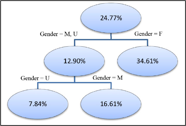
The following figure reconstructs the decision tree structure from the preceding fetched output:

Next let’s look at the distribution of the target variables and the measurement of the splits.
In [5]: output1[['_TreeLevel_', '_NodeID_', '_Parent_',
'_TargetVal0_', '_TargetVal1_', '_CI0_', '_CI1_',
'_Gain_', '_NumObs_']].sort_values('_NodeID_').head(20)
Out[5]:
Selected Rows from Table TREEMODEL1
_TreeLevel_ _NodeID_ _Parent_ _TargetVal0_ _TargetVal1_
0 0.0 0.0 -1.0 No Bought
1 1.0 1.0 0.0 No Bought
2 1.0 2.0 0.0 No Bought
3 2.0 3.0 1.0 No Bought
4 2.0 4.0 1.0 No Bought
_CI0_ _CI1_ _Gain_ _NumObs_
0 0.752284 0.247716 0.047713 1688948.0
1 0.870955 0.129045 0.012886 765624.0
2 0.653881 0.346119 0.000000 923324.0
3 0.921578 0.078422 0.000000 323684.0
4 0.833878 0.166122 0.000000 441940.0
The first row returns the overall frequency distribution of the response variable. In this case, the overall sample percentage of those who buy organic food is 24.77%. The decision tree algorithm then evaluates all possible ways to cut the entire data into two segments. Since we have only one predictor with three levels, there are only three ways to split the data into two segments:
● Gender = F versus Gender = M, U
● Gender = M versus Gender = F, U
● Gender = U versus Gender = F, M
The dtreetrain action evaluates all these three possible splits and selects the best one based on a certain criterion. The default criterion that is used by dtreetrain is information gain, which is the difference between of the entropy of the parent node and the weighted average of entropies of the child nodes. In other words, information gain tries to find a split that maximizes the difference of the target distribution between
the parent node and the child nodes. The best split chosen by dtreetrain is Gender = F versus Gender = M, U with information gain 0.0477. The sample percentage of those who buy organic food and who are the two children of node 0 is 12.90% and 34.61%, respectively.
The tree model continues to evaluate the splits on the two segments and to determine whether they can be further split. The continued evaluation for more splits is the reason why a decision tree is also known as a recursive partition. The tree structure is grown using recursive partitioning, until one of the following criteria is met:
● The current partition cannot be split anymore.
● The minimum leaf size has been reached.
● The maximum depth of the tree has been reached.
The following figure shows the final decision tree model that we have built:
The following table lists some important parameters for training a decision tree model:
| Parameter | Description | Default |
| maxbranch | Specifies the maximum number of children (branches) that are allowed for each level of the tree. | 2 |
| maxlevel | Specifies the maximum number of tree levels. | 6 |
| leafsize | Specifies the minimum number of observations on each node. | 1 |
| prune=True | False | Specifies whether to use a C4.5 pruning method for classification trees or minimal cost-complexity pruning for regression trees. | False |
| varimp=True | False | Specifies whether the variable importance information is generated. The importance value is determined by the total Gini reduction. | False |
| cflev | Specifies the aggressiveness of tree pruning according to the C4.5 method. |
The dtreetrain action supports the following criteria for evaluating the splits in a decision tree growing process:
| Parameter | Description |
| crit=chaid | CHAID (Chi-square Automatic Interaction Detector) technique |
| crit=chisquare | Chi-square test |
| crit=gain | Information gain |
| crit=gainratio | Information gain ratio |
| crit=gini | Per-leaf Gini statistic |
Building a decision tree model usually involves a pruning step after the tree is grown. You must enable the prune option to request dtreetrain to include an additional pruning step after the tree is grown.
In [6]: tree1.prune = True
...: tree1()
Out[6]:
[ModelInfo]
Decision Tree for ORGANICS
Descr Value
0 Number of Tree Nodes 3.000000e+00
1 Max Number of Branches 2.000000e+00
2 Number of Levels 2.000000e+00
3 Number of Leaves 2.000000e+00
4 Number of Bins 2.000000e+01
5 Minimum Size of Leaves 7.656240e+05
6 Maximum Size of Leaves 9.233240e+05
7 Number of Variables 1.000000e+00
8 Confidence Level for Pruning 2.500000e-01
9 Number of Observations Used 1.688948e+06
10 Misclassification Error (%) 2.477163e+01
[OutputCasTables]
casLib Name Rows Columns
0 CASUSERHDFS(username) treeModel1 3 24
casTable
0 CASTable('treeModel1', caslib='CASUS...
In [7]: output1[['_TreeLevel_', '_NodeID_', '_Parent_', '_ParentName_',
'_NodeType_', '_PBName0_',
'_PBName1_']].sort_values('_NodeID_').head(20)
Out[7]:
Selected Rows from Table TREEMODEL1
_TreeLevel_ _NodeID_ _Parent_ _ParentName_ _NodeType_
0 0.0 0.0 -1.0 1.0
1 1.0 1.0 0.0 DemGender 3.0
2 1.0 2.0 0.0 DemGender 3.0
_PBName0_ _PBName1_
0
1 M U
2 F
Compared to the code in In[2], Node 3 and Node 4 are pruned back according to the pruning criterion. The default pruning criterion is a modified C4.5 method, which estimates the error rate for validation data that is based on the classification error rate of the training data. The pruning criterion is not generated by the dtreetrain action. However, you can use the information gain output that is generated by the tree model without pruning in order to understand why this split is not significant (the information gain is 0.0129) compared to the first split (the information gain is 0.0477).
Pruning a decision tree is used to avoid model overfitting when you use the decision tree to score new data (validation data). The C4.5 method does not require validation data in order to prune a tree. If you do have holdout data, you can use the dtreeprune action to prune a given tree model.
data2 = conn.CASTable('your_validation_data')
output2 = conn.CASTable('pruned_tree')
data2.dtreeprune(model=output1, casout=output2)
Next let’s add more variables to the decision tree models.
In [8]: varlist = ['DemGender', 'DemHomeowner', 'DemAgeGroup', 'DemCluster', 'DemReg',
'DemTVReg', 'DemFlag1', 'DemFlag2', 'DemFlag3', 'DemFlag4', 'DemFlag5',
'DemFlag6', 'DemFlag7', 'DemFlag8', 'PromClass']
...:
...: output2 = conn.CASTable('treeModel2', replace=True)
...:
...: tree2 = organics.dtreetrain
...: tree2.target = 'TargetBuy'
...: tree2.inputs = varlist
...: tree2.casout = output2
...: tree2()
Out[8]:
[ModelInfo]
Decision Tree for ORGANICS
Descr Value
0 Number of Tree Nodes 4.300000e+01
1 Max Number of Branches 2.000000e+00
2 Number of Levels 6.000000e+00
3 Number of Leaves 2.200000e+01
4 Number of Bins 2.000000e+01
5 Minimum Size of Leaves 7.600000e+01
6 Maximum Size of Leaves 5.972840e+05
7 Number of Variables 1.500000e+01
8 Confidence Level for Pruning 2.500000e-01
9 Number of Observations Used 1.688948e+06
10 Misclassification Error (%) 2.389866e+01
[OutputCasTables]
casLib Name Rows Columns
0 CASUSERHDFS(username) treeModel2 43 130
casTable
0 CASTable('treeModel2', caslib='CASUS...
The ModelInfo output in the preceding example indicates that a larger decision tree has been grown. The new tree has 43 nodes and 22 of them are terminal nodes (leaves). The tree has 6 levels and the smallest leaves have 76 observations. For data with 1.7 million observations, sometimes, we might not be interested in subsets of data with only 76 observations. You can actually control subset size by the leafsize parameter. You can set leafsize to 1000 in order to grow a smaller tree, as follows:
In [9]: organics.dtreetrain(
...: target = 'TargetBuy',
...: inputs = varlist,
...: casout = output2,
...: leafSize = 1000,
...: maxLevel = 4,
...: )
Out[9]:
[ModelInfo]
Decision Tree for ORGANICS
Descr Value
0 Number of Tree Nodes 1.500000e+01
1 Max Number of Branches 2.000000e+00
2 Number of Levels 4.000000e+00
3 Number of Leaves 8.000000e+00
4 Number of Bins 2.000000e+01
5 Minimum Size of Leaves 1.216000e+03
6 Maximum Size of Leaves 8.891240e+05
7 Number of Variables 1.500000e+01
8 Confidence Level for Pruning 2.500000e-01
9 Number of Observations Used 1.688948e+06
10 Misclassification Error (%) 2.393466e+01
[OutputCasTables]
casLib Name Rows Columns
0 CASUSERHDFS(username) treeModel2 15 130
casTable
0 CASTable('treeModel2', caslib='CASUS...
In the previous example, the new decision tree produced only 15 nodes and 8 of them are leaves. Using this tree model to score a new observation is straightforward. You first identify the leaf node that contains this observation, and use the sample event probability of the node as the estimated event probability for that observation. The CAS decisiontree action set provides a dtreescore action for you to score a data set as well.
In [10]: organics.dtreescore(modelTable=conn.CASTable('treeModel2'))
Out[10]:
[ScoreInfo]
Descr Value
0 Number of Observations Read 1688948
1 Number of Observations Used 1688948
2 Misclassification Error (%) 23.934662287
The model option in dtreescore points to the tree model that we trained and stored on the CAS server, and it uses the model to score the ORGANICS CAS table. The dtreescore action in this example does not actually save the predictions to a new CAS table. You must use a casout option to save the predictions.
In [11]: output3 = conn.CASTable('predicted', replace=True)
...: organics.dtreescore(modelTable=output2, casout=output3)
...: output3.columns
Out[11]: Index(['_DT_PredName_', '_DT_PredP_', '_DT_PredLevel_', '_LeafID_', '_MissIt_', '_NumNodes_', '_NodeList0_', '_NodeList1_', '_NodeList2_', '_NodeList3_'], dtype='object')
In [12]: output3.head(10)
Out[12]:
Selected Rows from Table PREDICTED
_DT_PredName_ _DT_PredP_ _DT_PredLevel_ _LeafID_ _MissIt_
0 No 0.840345 0.0 8.0 1.0
1 No 0.667749 0.0 9.0 0.0
2 No 0.840345 0.0 8.0 0.0
3 No 0.667749 0.0 9.0 1.0
4 No 0.667749 0.0 9.0 1.0
5 No 0.559701 0.0 11.0 1.0
6 No 0.667749 0.0 9.0 1.0
7 No 0.840345 0.0 8.0 1.0
8 No 0.667749 0.0 9.0 0.0
9 No 0.923686 0.0 7.0 0.0
_NumNodes_ _NodeList0_ _NodeList1_ _NodeList2_ _NodeList3_
0 4.0 0.0 1.0 3.0 8.0
1 4.0 0.0 1.0 4.0 9.0
2 4.0 0.0 1.0 3.0 8.0
3 4.0 0.0 1.0 4.0 9.0
4 4.0 0.0 1.0 4.0 9.0
5 4.0 0.0 2.0 5.0 11.0
6 4.0 0.0 1.0 4.0 9.0
7 4.0 0.0 1.0 3.0 8.0
8 4.0 0.0 1.0 4.0 9.0
9 4.0 0.0 1.0 3.0 7.0
The following table summarizes the columns that are generated as output by a dtreescore action.
| Output Column | Description |
| _DT_PredName_ | The predicted value, which is the most frequent level of the leaf that the observation is assigned to. |
| _DT_PredP_ | The predicted probability, which is equal to the sample frequency of the predicted value in the leaf that the observation is assigned to. |
| _DT_PredLeveL_ | The index of the predicted value. If the response variable has k levels, this column takes values from 0, 1, ..,k – 1 |
| _LeafID_ | The node ID of the leaf that the observation is assigned to. |
| _MissIt_ | The indicator for misclassification. |
| _NumNodes__NodeListK_ | _NumNodes_ indicates the depth of the leaf. The list of _NodeListK_ variables stores the path from the root node to the current leaf. |
Gradient Boosting, Forests, and Neural Networks
The decisiontree action set also contains the actions for building gradient boosting and random forest models. Unlike decision trees, gradient boosting and random forests are machine-learning techniques that produce predictions that are based on an ensemble of trees. Gradient boosting models are usually based on a set of weak prediction models (small decision trees or even tree stumps). By contrast, random forests are usually based on a set of full grown trees (deep trees) on subsample data. Another major difference is that gradient boosting grows decision trees sequentially and a random forest grows decision trees in parallel. For more details about tree models, refer to [1] and [2] at the end of the chapter.
Both gradient boosting and random forest models are available in the decisiontree action set through three distinct actions that cover basic steps of a machine learning pipeline: model training, scoring, and delivery (score code generation).
In [1]: conn.help(actionset='decisiontree')
NOTE: Added action set 'decisiontree'.
Out[1]:
decisionTree
decisionTree
Name Description
0 dtreeTrain Train Decision Tree
1 dtreeScore Score A Table Using Decision Tree
2 dtreeSplit Split Tree Nodes
3 dtreePrune Prune Decision Tree
4 dtreeMerge Merge Tree Nodes
5 dtreeCode Generate score code for Decision Tree
6 forestTrain Train Forest
7 forestScore Score A Table Using Forest
8 forestCode Generate score code for Forest
9 gbtreeTrain Train Gradient Boosting Tree
10 gbtreeScore Score A Table Using Gradient Boosting Tree
11 gbtreecode Generate score code for Gradient Boosting Trees
Let’s first train a simple random forest model using the Organics data set to predict the probability of buying organic food.
In[2]: varlist = ['DemGender', 'DemHomeowner', 'DemAgeGroup',
'DemCluster', 'DemReg', 'DemTVReg', 'DemFlag1',
'DemFlag2', 'DemFlag3', 'DemFlag4', 'DemFlag5',
'DemFlag6', 'DemFlag7', 'DemFlag8', 'PromClass']
...:
...: output = conn.CASTable('forest1', replace=True)
...:
...: forest1 = organics.Foresttrain()
...: forest1.target = 'TargetBuy'
...: forest1.inputs = varlist
...: forest1.casout = output
...: forest1()
Out[2]:
[ModelInfo]
Forest for ORGANICS
Descr Value
0 Number of Trees 50.000000
1 Number of Selected Variables (M) 4.000000
2 Random Number Seed 0.000000
3 Bootstrap Percentage (%) 63.212056
4 Number of Bins 20.000000
5 Number of Variables 15.000000
6 Confidence Level for Pruning 0.250000
7 Max Number of Tree Nodes 57.000000
8 Min Number of Tree Nodes 19.000000
9 Max Number of Branches 2.000000
10 Min Number of Branches 2.000000
11 Max Number of Levels 6.000000
12 Min Number of Levels 6.000000
13 Max Number of Leaves 29.000000
14 Min Number of Leaves 10.000000
15 Maximum Size of Leaves 927422.000000
16 Minimum Size of Leaves 10.000000
17 Out-of-Bag MCR (%) NaN
[OutputCasTables]
casLib Name Rows Columns
0 CASUSERHDFS(username) forest1 2280 132
casTable
0 CASTable('forest1', caslib='CASUSERH...
The foresttrain action returns two result tables to the client: ModelInfo and OutputCasTables. The first table contains parameters that define the forest, parameters that define each individual tree, and tree statistics such as the minimum and maximum number of branches and levels. A forest model is an ensemble of homogenous trees, with each tree growing on a different subset of the data (usually from bootstrap sampling). Therefore, the size and depth of the trees might be different from each other even though the tree parameters that you define are the same. The idea of a forest is to grow a deep tree on each subsample in order to produce “perfect” predictions for the local data (low bias but high variance) and then use the ensemble technique to reduce the overall variance.
Some key parameters that define a random forest model are listed in the following table. The foresttrain action also enables you to configure the individual trees, and the parameters are identical to those in the dtreetrain action. In general, you must grow deep trees for each bootstrap sample, and pruning is often unnecessary.
| Parameter | Description |
| ntree | The number of trees in the forest ensemble, which is 50, by default. |
| m | The number of input variables to consider for splitting on a node. The variables are selected at random from the input variables. By default, forest uses the square root of the number of input variables that are used, rounded up to the nearest integer. |
| vote=’majority’ | Uses majority voting to collect the individual trees into an ensemble. This is the default ensemble for classification models. |
| vote=’prob’ | Uses the average of predicted probabilities or values to collect the individual trees into an ensemble. |
| seed | The seed that is used for the random number generator in bootstrapping. |
| bootstrap | Specifies the fraction of the data for the bootstrap sample. The default value is 0.63212055882. |
| oob | The Boolean value to control whether the out-of-bag error is computed when building a forest. |
Random forest models are also commonly used in variable selection, which is usually determined by the variable importance of the predictors in training the forest model. The importance of a predictor to the target variable is a measure of its overall contribution to all the individual trees. In the foresttrain action, this contribution is defined as the total Gini reduction from all of the splits that use this predictor.
In [3]: forest1.varimp = True
...: result = forest1()
...: result['DTreeVarImpInfo']
...:
Out[3]:
Forest for ORGANICS
Variable Importance Std
0 DemGender 16191.631365 7820.237986
1 DemAgeGroup 7006.819480 2827.738946
2 PromClass 2235.407366 1199.868546
3 DemTVReg 288.048039 68.934845
4 DemFlag2 249.873589 253.060732
5 DemFlag6 226.131347 309.079859
6 DemCluster 222.589229 70.478049
7 DemFlag1 162.256557 177.508653
8 DemReg 114.090856 50.533349
9 DemFlag7 40.931939 35.704581
10 DemFlag5 8.986376 23.494624
11 DemFlag4 8.583654 17.210787
12 DemFlag8 6.291225 12.721568
13 DemFlag3 5.888663 23.692049
14 DemHomeowner 0.446454 0.812748
The foresttrain action also produces an OutputCasTables result table, which contains the name of the CAS table that stores the actual forest model. The CAS table, which is stored on the CAS server, describes all the individual trees. Each row of this CAS table contains the information about a single node in an individual tree. When you have a large of number of trees, this table can be large, and therefore, is stored on the CAS server instead. In the preceding example, the forest model contains 50 trees and 2278 nodes, in total being returned to the client.
In [4]: result['OutputCasTables']
Out[4]:
casLib Name Rows Columns
0 CASUSERHDFS(usrname) forest1 2278 132
casTable
0 CASTable('forest1', caslib='CASUSERH...
casLib Name Rows Columns
0 CASUSERHDFS(username) forest1 2278 132
To score the training data or the holdout data using the forest model, you can use the forestscore action.
scored_data = conn.CASTable('scored_output', replace=True)
organics.forestscore(modelTable=conn.CASTable('forest1'), casout=scored_data)
Unlike the random forest model, gradient boosting grows trees sequentially, whereby each tree is grown based on the residuals from the previous tree. The following example shows how to build a gradient boosting model using the same target and predictors as in the forest model.
In [5]: varlist = ['DemGender', 'DemHomeowner', 'DemAgeGroup', 'DemCluster',
'DemReg', 'DemTVReg', 'DemFlag1', 'DemFlag2', 'DemFlag3',
'DemFlag4', 'DemFlag5', 'DemFlag6', 'DemFlag7', 'DemFlag8',
'PromClass']
...:
...: output = conn.CASTable('gbtree1', replace=True)
...:
...: gbtree1 = organics.Gbtreetrain()
...: gbtree1.target = 'TargetBuy'
...: gbtree1.inputs = varlist
...: gbtree1.casout = output
...: gbtree1()
...:
...:
Out[5]:
[ModelInfo]
Gradient Boosting Tree for ORGANICS
Descr Value
0 Number of Trees 50.0
1 Distribution 2.0
2 Learning Rate 0.1
3 Subsampling Rate 0.5
4 Number of Selected Variables (M) 15.0
5 Number of Bins 20.0
6 Number of Variables 15.0
7 Max Number of Tree Nodes 63.0
8 Min Number of Tree Nodes 61.0
9 Max Number of Branches 2.0
10 Min Number of Branches 2.0
11 Max Number of Levels 6.0
12 Min Number of Levels 6.0
13 Max Number of Leaves 32.0
14 Min Number of Leaves 31.0
15 Maximum Size of Leaves 512468.0
16 Minimum Size of Leaves 33.0
17 Random Number Seed 0.0
[OutputCasTables]
casLib Name Rows Columns
0 CASUSERHDFS(username) gbtree1 3146 119
casTable
0 CASTable('gbtree1', caslib='CASUSERH...
The following table lists the key parameters to grow a sequence of trees in a gradient boosting model. The gbtreetrain action also enables you configure the individual trees. These parameters are identical to those in the dtreetrain action.
| Parameter | Description |
| ntree | The number of trees in the gradient boosting model. The default is 50. |
| m | The number of input variables to consider for splitting on a node. The variables are selected at random from the input variables. By default, all input variables are used. |
| seed | The seed for the random number generator for sampling. |
| subsamplerate | The fraction of the subsample data to build each tree. The default is 0.5. |
| distribution | The type of gradient boosting tree to build. The value 0 is used for a regression tree, and 1 is used for a binary classification tree. |
| lasso | The L1 norm regularization on prediction. The default is 0. |
| ridge | The L2 norm regularization on prediction. The default is 0. |
To score the training data or the holdout data using the gradient boosting model, you can use the gbtreescore action.
scored_data = conn.CASTable('scored_output', replace=True)
organics.gbtreescore(modelTable=conn.CASTable('gbtree1'), casout=scored_data)
Neural networks are machine learning models that derive hidden features (neuron) as nonlinear functions of linear combination of the predictors, and then model the target variable as a nonlinear function of the hidden features. Such nonlinear transformations are often called activation functions in neural networks. The following figure illustrates a simple neural network between three predictors and a binary target that takes levels 0 and 1. In this case, there are four hidden features. Each is a nonlinear function of the linear combination of the three predictors. The probabilities of target = 1 and target = 0 are modeled as a nonlinear function of the hidden features. In neutral networks, such hidden features are called neurons, and it is common to have more than one layer of hidden neurons.

The neural network of related actions is available in the neuralnet action set. Let’s load the action set and continue to use the Organics data set to build a simple neural network.
In [6]: conn.loadactionset('neuralnet')
...: conn.help(actionset='neuralnet')
...:
NOTE: Added action set 'neuralNet'.
NOTE: Information for action set 'neuralNet':
NOTE: neuralNet
NOTE: annTrain - Train an artificial neural network
NOTE: annScore - Score a table using an artificial neural network model
NOTE: annCode - Generate DATA step scoring code from an artificial neural network model
In [7]: neural1 = organics.Anntrain()
...: neural1.target = 'TargetBuy'
...: neural1.inputs = ['DemAge','DemAffl','DemGender']
...: neural1.casout = output
...: neural1.hiddens = [4,2]
...: neural1.maxIter = 500
...: result = neural1()
...: list(result.keys())
Out[7]: ['OptIterHistory', 'ConvergenceStatus', 'ModelInfo', 'OutputCasTables']
In this case, we built a neural network with two layers. The first layer has four hidden neurons and the second layer has two hidden neurons. The maximum number of iterations for training the neural network is set to 500. The iteration history and convergence status of the model are reported in OptIterHistory and ConvergenceStatus result tables, respectively. The ModelInfo result table contains basic information about the neural network model:
In [8]: result['ModelInfo']
Out[8]:
Neural Net Model Info for ORGANICS
Descr Value
0 Model Neural Net
1 Number of Observations Used 1498264
2 Number of Observations Read 1688948
3 Target/Response Variable TargetBuy
4 Number of Nodes 13
5 Number of Input Nodes 5
6 Number of Output Nodes 2
7 Number of Hidden Nodes 6
8 Number of Hidden Layers 2
9 Number of Weight Parameters 30
10 Number of Bias Parameters 8
11 Architecture MLP
12 Number of Neural Nets 1
13 Objective Value 1.7011968247
The default error function of the anntrain action is NORMAL for continuous target or ENTROPY for categorical target. The anntrain action also provides parameters for customizing the neural networks such as the error function, the activation function, and the target activation function. Some key parameters of the anntrain action are listed in the following table:
| Parameter | Description |
| arch | Specifies the architecture of the network. arch = ‘MLP’: The standard multilayer perceptron network. arch =’GLIM’: The neural network with no hidden layer. arch = ‘DIRECT’: The MLP network with additional direct links from input nodes to the target nodes. |
| errorfunc | Specifies the error function for training the neural network. ENTROPY is available for categorical target. GAMMA, NORMAL, and POISSON are available for continuous targets. |
| targetact | Specifies the target activation function that links the hidden neurons at the last layer to the target nodes. LOGISTIC and SOFMAX (default) are available for categorical targets. EXP, IDENTITY, SIN, and TANH (default) are available for continuous targets. |
| act | Specifies the activation function that links the input nodes to the hidden neurons at the first layer, or neurons from one layer to the next layer. Available activation functions include EXP, IDENTITY, LOGISTIC, RECTIFIER, SIN, SOFTPLUS, and TANH (default). |
| targetcomb | Specifies the way to combine neurons in the target activation function. Linear combination (LINEAR) is the default. Other combinations are additive (ADD) and radial (RADIAL). |
| comb | Specifies the way to combine neurons or read as input in the activation functions. Linear combination (LINEAR) is the default. Other combinations are Additive (ADD) and radial (RADIAL). |
| ntries | The number of tries for random initial values of the weight parameters. |
| includebias | Indicates whether to include the intercept term (usually called bias) in the combination function. This parameter is ignored if an additive combination is used. Additive combinations are Combination (comb) and Target Combination (targetComb). |
Similar to the tree models in CAS, a CAS table in the server can be used for storing the neural network model. This is convenient when you build a large neural network and it avoids the I/O traffic between the Python client and the CAS server. To score a data set that uses a CAS table and that contains the neural network model, you can use the annscore action.
In [9]: organics.annscore(modelTable=output)
...:
Out[9]:
[ScoreInfo]
Descr Value
0 Number of Observations Read 1688948
1 Number of Observations Used 1498264
2 Misclassification Error (%) 18.448818099
Conclusion
In this chapter, we introduced several analytic models that are available on the CAS server for modeling categorical variables. This includes the logistic regression in the regression action set, the tree family (decision tree, random forest, gradient boosting) in the decisiontree action set, and simple neural networks in the neuralnet action set. For more information about the models, see the following references.
[1] Friedman, Jerome, Trevor Hastie, and Robert Tibshirani. 2001. The Elements of Statistical Learning. Vol. 1. Springer, Berlin: Springer Series in Statistics.
[2] Breiman, Leo. 2001. "Random Forests." In Machine Learning 45.1:5-32.