Appendix A: A Crash Course in Python
Plotting from Pandas DataFrame Methods
Plotting DataFrames using Plotly and Cufflinks
Creating Graphics with Matplotlib
Interactive Visualization with Bokeh
We expect that you have some familiarity with Python or you have at least some programming experience. We do not attempt to teach you everything about Python because there are many good books already out there for that purpose, However, we do want to briefly cover the major features that are necessary to take full advantage of the packages that are covered in this book.
IPython and Jupyter
Our first topic is which environment you would like to work in. With Python, you have many choices. You can use the standard Python interactive interpreter, which is quite nice compared to many other scripting language interpreters, but there are other choices that you might find even better.
A step up from the standard Python interpreter is the IPython interpreter. It starts from a command line just like the normal Python interpreter, but it includes some nice features that enhance interactive use. Features include tab completion of methods and attributes on objects, easy access to documentation strings, automatic display of results, and input and output history. Here is a brief demonstration of the ipython shell.
% ipython
Python 3.4.1 (default, Jun 3 2014, 16:31:42)
Type "copyright", "credits" or "license" for more information.
IPython 3.0.0 -- An enhanced Interactive Python.
? -> Introduction and overview of IPython's features.
%quickref -> Quick reference.
help -> Python's own help system.
object? -> Details about 'object', use 'object??' for extra details.
In [1]: a = 'hello'
In [2]: b = 'world'
In [3]: a + ' ' + b
Out[3]: 'hello world'
In [4]: Out[3]
Out[4]: 'hello world'
In [5]: In[3]
Out[5]: "a + ' ' + b"
In [6]: a
Out[6]: 'hello'
IPython also has a web-based notebook interface called Jupyter, which was previously known as IPython notebook. This notebook includes the same behaviors as the IPython shell, but with an attractive web interface. The web interface enables Python objects to be displayed graphically inline with the code. In addition, you can document your code in the notebook as well with formatted text, equations, and so on. Notebooks can be saved in their own format for use later or for sharing with others, or they can be exported to formats such as HTML for publishing on the web. You can start the notebook interface with the command jupyter notebook, or you can start it on Windows from the Anaconda menu.

In addition to IPython and Jupyter, there are more formal integrated development environments such as Spyder, Canopy, and Wing that include better support for editing multiple Python files and debugging. As you get more experienced writing Python programs, these might be more useful. For this book, we will primarily use the IPython shell. When we get into sections where a more graphical output is beneficial, we will switch to using Jupyter.
Data Types and Collections
In any type of data science, data types become an important topic. Python has a rich data type system, which maps well to the rectangular data sets that we work with in CAS.
Numeric Data Types
The most common data types that we use are integers, floating-point numbers, and character data. Python has objects for integers (int and long (in Python 2)) and floating-point values (float).
In [7]: type(100)
Out[7]: int
In [8]: type(1.0)
Out[8]: float
When you start working with the Pandas or NumPy packages, you might encounter some alternative implementations of numeric values. They work transparently as Python numeric values, so unless you are doing something more advanced, you don’t need to be concerned about them.
In [9]: import pandas as pd
In [10]: ser = pd.Series([100, 200])
# Pandas and Numpy use custom numeric types
In [11]: type(ser[0])
Out[11]: numpy.int64
# They still work as normal numeric values though
In [12]: ser[0] + 1000
Out[12]: 1100
Character Data Types
Python also has two different types of objects for character data that differ according to the version of Python used. In Python 2, the default string type is str and is a string of arbitrary bytes. The unicode object is for character data that contains text.
In Python 3, the default string type changed to unicode, and byte strings are represented using the bytes type. In either version, you can force a literal string to be represented in Unicode by preceding the string with the prefix “u”. Byte strings can be forced by using the prefix “b”. Each of these prefixes must be in lowercase. In either case, you can use double quotation marks or single quotation to enclose the string. The following code shows the Python 3 types of various strings.
In [13]: type('hello')
Out[13]: str
In [14]: type(u'hello')
Out[14]: str
In [15]: type(b' world')
Out[15]: bytes
In [16]: u'hello' + b' world'
---------------------------------------------------------------------------
TypeError Traceback (most recent call last)
<ipython-input-64-0af8b45d0f72> in <module>()
----> 1 u'hello' + b' world'
TypeError: Can't convert 'bytes' object to str implicitly
In [17]: u'hello' + b' world'.decode('utf-8')
Out[17]: 'hello world'
Although the distinction between the two doesn’t seem significant here, and both types seem to act the same, issues can arise when you include non-ASCII characters in your strings. If you put non-ASCII text in a byte string, Python has no knowledge of the encoding of those bytes. Examples of encoding are latin-1, utf-8, windows-1252, and so on. Also, your system’s default encoding might cause the display of different characters than you expect when they are printed. Because of this, when you store text in variables, you should always use unicode objects. Byte strings should be used only for binary data.
Booleans
Although Python has a system to make nearly every variable act like a Boolean (for example, 1 and “hello” are true, whereas 0 and “” are false), it is best to use the explicit True and False values when possible. The use of explicit values is especially important when interacting with another system such as CAS, which might have different rules for casting values to Booleans.
Lists and Tuples
The first collection type that we look at is the list. A list is an ordered collection of any type of object. Unlike array types in many languages, Python lists can contain a mixture of object types. Another nice feature of lists is that they are mutable.
Lists can be specified explicitly using items that are enclosed in brackets. They are also zero-indexed, which means that the first index of the list is zero.
In [18]: items = ['a', 'b', 'c', 100]
In [19]: items
Out[19]: ['a', 'b', 'c', 100]
In [20]: items[0]
Out[20]: 'a'
In [21]: items[2]
Out[21]: 'c'
Another nice feature of lists is that they can be indexed using negative numbers. Negative numbers indicate indexes from the end of the list. So a -1 index returns the last item in a list, and a -3 returns the third item from the end of the list.
In [22]: items[-1]
Out[22]: 100
In [23]: items[-3]
Out[23]: 'b'
Slicing
In addition to retrieving single items, you can also retrieve slices of lists. Slicing is done by specifying a range of indexes.
In [24]: items[1:3]
Out[24]: ['b', 'c']
In the preceding code, we specify a slice from 1 to 3. A slice of a list includes the range of items from the initial index, up to (but not including) the last index. So this example returns a new list that includes items 1 and 2. If the first index in the slice is left empty, the slice includes everything to the beginning of the list. Accordingly, if the last index in the slice is empty, everything to the end of the list is included.
A third component of a slice can be given to specify a step size. For example, the following code returns every other item in the list starting with the first item.
In [25]: items[::2]
Out[25]: ['a', 'c']
In the following example, we get every other item in the list starting with the second item.
In [26]: items[1::2]
Out[26]: ['b', 100]
It is also possible to specify negative step sizes to step in reverse. But using negative step sizes with start and end points can get confusing. If you need to step in reverse, it might be a good idea to do that in a separate step.
Tuples
Tuples and lists behave nearly the same. The primary difference is that tuples are not mutable. Once a tuple has been created, it cannot be modified. Indexing and slicing works the same way except that slicing returns a new tuple rather than a list. Tuples are mostly used by Python internally, but you can specify them explicitly just like lists, except that you use parentheses to enclose the items.
In [27]: items = ('a', 'b', 'c', 100)
In [28]: items
Out[28]: ('a', 'b', 'c', 100)
One reason that you might need a tuple rather than a list is that lists cannot be used as a key in a dictionary or as an item of a set. Those data types are discussed in the next section.
Dictionaries and Sets
Dictionaries and sets are used to hold unordered collections of items. Dictionaries contain both a key and a value. The keys must be unique, and each one points to a stored value, which doesn’t have to be unique. Sets are simply collections of unique items. You can think of them as a set of dictionary keys without associated values.
Dictionaries can be built using any of these methods: dictionary literal syntax, the dict constructor, or one key/value pair at a time. The following code demonstrates each of those methods.
# Dictionary literal
In [29]: pairs = {'key1': 100, 'key2': 200, 'key3': 400}
In [30]: pairs
Out[30]: {'key1': 100, 'key2': 200, 'key3': 400}
# Using the dict constructor
In [31]: pairs = dict(key1=100, key2=200, key3=400)
In [32]: pairs
Out[32]: {'key1': 100, 'key2': 200, 'key3': 400}
# Adding key / value pairs one at a time
In [33]: pairs['key4'] = 1000
In [34]: pairs['key5'] = 2000
In [35]: pairs
Out[35]: {'key1': 100, 'key2': 200, 'key3': 400, 'key4': 1000, 'key5': 2000}
Although we have used strings for all of the keys in these examples, you can use any immutable object as a key. Values can be any object, mutable or immutable. The only catch is that if you use the dict constructor with keywords as we did in the preceding example, your keys will always have to be valid variable names, which are converted strings.
Accessing the value of a key is just like accessing the index of a list. The difference is that you specify the key value rather than an index.
In [36]: pairs['key4']
Out[36]: 1000
In addition to accessing keys explicitly, you can get a collection of all of the keys or values of a dictionary using the keys and values methods, respectively.
In [37]: pairs.keys()
Out[37]: dict_keys(['key1', 'key3', 'key2', 'key5', 'key4'])
In [38]: pairs.values()
Out[38]: dict_values([100, 400, 200, 2000, 1000])
Depending on which version of Python you use, you might see something slightly different. Python 3 returns an iterable view of the elements, whereas Python 2 returns a list of the elements. Each version of Python has behaviors that are different from the other, but most of the time the result of the keys and values methods are used to iterate through elements in a dictionary and act consistently in that context, which we see in the next section.
Sets
As we mentioned, sets act like a set of dictionary keys without the values, including the fact that every element must be unique. In fact, the literal syntax for sets even looks like a dictionary literal without values.
In [39]: items = {100, 200, 400, 2000, 1000}
In [39]: items
Out[39]: {100, 200, 400, 1000, 2000}
You can also use the set constructor to build sets, much like you would a dictionary using the dict constructor. The set constructor takes an iterable object, usually a list, as an argument rather than multiple arguments. Or you can add items individually using the add method.
In [40]: items = set(['key1', 'key2', 'key3'])
In [41]: items
Out[41]: {'key1', 'key2', 'key3'}
In [42]: items.add('key4')
In [42]: items.add('key5')
In [43]: items
Out[43]: {'key1', 'key2', 'key3', 'key4', 'key5'}
Sets have many interesting operations that can be used to find the common elements or differences between them and other sets, but they are also used fairly often in iteration. We won’t go any deeper into sets here, but we will show how they are used in a looping context in the section about flow control.
Other Types
Python’s type system is very rich, so we couldn’t possibly touch on all of the built-in types that Python supplies much less the types that programmers can create themselves. For more information about Python’s built-in types, you can read the types Python package documentation.
Flow Control
Flow control includes conditional statements and looping. Python uses if, elif, and else statements for conditional blocks. Looping uses for or while statements.
Conditional Code
Python’s conditional statements work much like conditionals in other programming languages. The if statement starts a block of code that gets executed only if the condition that is specified in the if statement evaluates to True.
In [44]: value = 50
In [45]: if value >= 30:
....: print('value is sufficient')
....:
value is sufficient
In [46]: value = 20
In [47]: if value >= 30:
....: print('value is sufficient')
....:
Note that in the second if block, nothing was printed because the code inside the if block did not execute. You can also add an else block to have code execute when the condition isn’t true.
In [48]: if value >= 30:
....: print('value is sufficient')
....: else:
....: print('value is not sufficient')
....:
value is not sufficient
For cases in which you have multiple code blocks that each depend on a different condition, you use the elif statement after the initial if.
In [49]: value = 26
In [50]: if value >= 30:
....: print('value is sufficient')
....: elif value > 25:
....: print('getting closer')
....: elif value > 22:
....: print('not there yet')
....: else:
....: print('value is insufficient')
....:
getting closer
In any case, only the first block of code with a true condition is executed. Even if the conditions in the following elifs are true, they are ignored.
In addition to the simple conditions shown in the preceding example, compound conditions can be constructed by combining simple conditions with the and operator and the or operator. For example, to specify a condition that checks on whether a value is in the range of 20 to 30, including the endpoints, you use value >= 20 and value <=30. Such conditions can also be used in looping constructs, which we show next.
Looping
Python has two looping statements: while and for. The while loop is a lot like an if block except that the code within the block executes over and over again until the condition in the while statement is false. The for loop is used for iterating over collections or objects that support the Python iterator interface. Let’s look at while loops first since they are so similar to if blocks.
While Loops
The most important thing to remember about while loops is that you need to update the variables used in the while loop’s condition, or you must have another way of escaping the loop. Otherwise, you end up in an infinite loop. Here is a basic example that increments value until it reaches a specified value.
In [51]: value = 1
In [52]: while value < 5:
....: print(value)
....: value = value + 1
....:
1
2
3
4
Since an empty list (or a dictionary or a set) is considered to be a false value, you can use while loops to loop over elements in a list, as well.
In [53]: items = [100, 200, 300]
In [54]: while items:
....: print(items.pop())
....:
300
200
100
In this case, we modify the list as we loop by removing the last item of the list in each iteration. To preserve the list, you can make a copy of it before using the while loop, or you can use the for loop. Let’s look at that in the next section.
For Loops
Unlike for loops in most other languages, the Python for loop doesn’t use a specified condition to stop the looping. It is used to loop over collections or other objects that support Python’s iterator interface. The most basic use of the Python for loop is looping over a range of numbers supplied by the range function.
Depending on your Python version, the range function returns a list of integers (Python 2) or an iterable that iterates over a series of integers (Python 3). They both work the same way in the context of a for loop, though. Here is an example of this type of for loop.
In [55]: for i in range(5):
....: print(i)
....:
0
1
2
3
4
With a single argument, the range function generates values from zero up to (but not including) the value that is specified. Just as with slicing collections, you can specify a starting value, an ending value, and a step size in the range function.
# Count from 2 up to 6
In [56]: list(range(2,6))
Out[56]: [2, 3, 4, 5]
# Count from 2 up to 6 with a step size of 2
In [57]: list(range(2,6,2))
Out[57]: [2, 4]
Although looping over numeric ranges can be useful, looping over arbitrary collections and iterators is a more common operation. To loop over all of the items in a list, you simply specify that list as the loop variable.
In [58]: items = [100, 200, 300]
In [58]: for i in items:
....: print(i)
....:
100
200
300
Looping over dictionaries and sets works the same way. However, for dictionaries, the value that gets set at each iteration is the key name.
In [59]: pairs = {'key1': 100, 'key2': 200, 'key3': 300}
In [59]: for key in pairs:
....: print(key)
....:
key1
key3
key2
To iterate over values, you specify pairs.values() as the looping variable. Another common way to loop over dictionaries is by the key/value pairs. This is done with the items method.
In [60]: for key, value in pairs.items():
....: print('%s : %s' % (key, value))
....:
key1 : 100
key3 : 300
key2 : 200
Loop Controls
Most of the time, when looping, you continue to loop through all of the objects in the collection. However, there are times when you want to break out of a loop or you just want to skip to the next item in the loop. These are handled by the break and continue statements, respectively.
To break out of a loop completely, you use the break statement.
In [61]: for value in items:
....: if value > 150:
....: break
....: print(value)
100
If you hit a condition in a loop at which you simply want to go to the next item, you use the continue statement.
In [62]: for value in items:
....: if value == 200:
....: continue
....: print(value)
100
300
Looping Helper Functions
In addition to looping control statements, Python has several iterator helper functions. A couple of the most common ones are the enumerate and zip functions. The enumerate function enables you to iterate over items while also returning the index of the iteration. This prevents you from having to keep track of the iteration index yourself.
In [63]: for i, value in enumerate(items):
....: print(i, value)
0 100
1 200
2 300
The zip function enables you to loop over multiple parallel iterators at once.
In [64]: labels = ['a', 'b', 'c']
In [65]: for label, value in zip(labels, items):
....: print(label, value)
a 100
b 200
c 300
There are many intricacies of looping in Python that we won’t get into here, but the information here should be sufficient to cover the cases that we use in this book.
Functions
As in many other programming languages, functions enable you to group a set of statements together in an object that you can call multiple times in your program. They commonly accept arguments in order to send in data or options to modify the behavior of the operation. Python functions (and instance methods, which we discuss later) are defined using the def statement. The def statement takes a function name and zero or more parameters that are enclosed in parentheses. The content of the function is specified in an indented block after the def statement. Let’s look at a simple function with no arguments:
In [61]: def print_hello():
....: print('hello')
....:
In [62]: print_hello()
hello
In this function, we just print the word “hello”. If we want to customize the printed message, we can add a name argument to the function definition.
In [63]: def print_hello(name):
....: print('hello %s' % name)
....:
In [64]: print_hello('Kevin')
hello Kevin
In addition to positional arguments, Python also provides keyword arguments. In the following example, we use a keyword argument to control some optional behavior within the function. The excited keyword argument specifies a default value of False and determines whether the printed message contains an exclamation point or a period.
In [65]: def print_hello(name, excited=False):
....: if excited:
....: print('hello %s!' % name)
....: else:
....: print('hello %s.' % name)
....:
In [66]: print_hello('Kevin')
hello Kevin.
In [67]: print_hello('Kevin', excited=True)
hello Kevin!
In [68]: print_hello('Kevin', True)
hello Kevin!
The last call to print_hello in the preceding code also demonstrates that keyword argument values can be specified as positional arguments. The order in which the keyword arguments are defined determines the order in which they must be specified in the function call. You can also specify all arguments as keywords if you want to specify them in random order.
In [69]: print_hello(excited=True, name='Kevin')
hello Kevin!
In addition to performing operations, functions can also return values using the return statement.
In [70]: def print_hello(name):
....: return 'hello %s' % name
....:
In [71]: print_hello('Kevin')
Out[71]: 'hello Kevin'
If you don’t return a value, a value of None is returned.
An interesting aspect about functions is that they are variables just like the other variable types that we previously discussed. This means that the function definitions themselves can be passed as arguments, can be stored in collections, and so on. We use this technique in other locations in the book. To demonstrate that functions are Python objects, we display the type of our function here, add it to a list, and call it from the list directly.
In [72]: type(print_hello)
Out[72]: function
In [73]: a = [print_hello]
In [74]: a[0]
Out[74]: <function __main__.print_hello>
In [75]: a[0]('Kevin')
Out[75]: 'hello Kevin'
Constructing Arguments Dynamically
When working with our function example, we specified all of the arguments (both positional and keyword) explicitly. There are times when you want to construct arguments programmatically, and then call a function using the dynamically constructed arguments. Python does this with the * and ** operators. The * operator expands a list of items into positional arguments. The ** operator expands a dictionary into a set of keyword arguments. Let’s look at this example from the previous section again.
print_hello('Kevin', excited=True)
Rather than specifying the arguments explicitly, let’s build a list and a dictionary that contain the arguments, and use the * and ** operators to apply them to a function.
In [76]: positional = ['Kevin']
In [77]: keyword = {'excited': True}
In [78]: print_hello(*positional, **keyword)
hello Kevin!
As with looping, there are many details that we have glossed over in this section on functions. For a more detailed description of functions, refer to any one of the many books and web pages about Python that are readily available.
Classes and Objects
Classes and objects are large topics in Python that we do not explore deeply in this book. Although we use many classes and objects in the book, defining classes is not something that is commonly required in order to use the Python interface to CAS. Class definitions in Python use the class statement and generally contain multiple method definitions created by the def statement. Here is a sample class definition for a bank account:
class BankAccount(object):
def __init__(self, name, amount=0):
self.name = name
self.balance = amount
def report(self):
print('%s : $%.2f' % (self.name, self.balance))
def deposit(self, amount):
self.balance = self.balance + amount
def withdraw(self, amount):
self.balance = self.balance - amount
In this class, we do not inherit from another class other than Python’s base object as seen in the class statement. We have several methods defined that act on the account for depositing money, withdrawing money, and so on. There is one special method in this example called __init__. This is the constructor for the class that typically initializes all of the instance variables that are stored in the self variable. As you can see in all of the method definitions, the instance object self must be specified explicitly. Specifying the instance object in Python is unlike some other programming languages that implicitly define an instance variable name for you.
Creating an instance of a BankAccount object is done by calling it as if it were a function, while supplying the arguments that are defined in the constructor. Once you have an instance stored into a variable, you can operate on it using the defined methods. Here is a quick example:
In [76]: ba = BankAccount('Kevin', 1000)
In [77]: ba.report()
Kevin : $1000.00
In [78]: ba.deposit(500)
In [79]: ba.report()
Kevin : $1500.00
In [80]: ba.withdraw(200)
In [81]: ba.report()
Kevin : $1300.00
This might be the most brief description of Python classes that you ever see. However, as we mentioned earlier, defining classes while using the Python client to CAS is uncommon. Therefore, complete knowledge about them isn’t necessary.
Exceptions
Exceptions occur in programs when some event has occurred that prevents the program from going any further. Examples of such events are as simple as the division of a number by zero, a network connection failure, or a manually triggered keyboard interruption. Python defines dozens of different exception types, and package writers can add their own. To quickly demonstrate what happens when an exception occurs, you can run the following code:
In [82]: 100 / 0
---------------------------------------------------------------------------
ZeroDivisionError Traceback (most recent call last)
<ipython-input-72-a187b7beb4f1> in <module>()
----> 1 100 / 0
ZeroDivisionError: division by zero
In this case, the ZeroDivisionError exception was raised. Python enables you to capture exceptions after they have been raised so that you can handle the issue more gracefully. This is done using the try statement and the except statement. Each contains a block of code. The try block contains the code that you run that might raise an exception. The except block contains the code that gets executed if an exception is raised. Here is the most basic form:
In [83]: try:
....: 100 / 0
....: except:
....: print('An error occurred')
....:
An error occurred
As you can see, we prevent the continuation of the ZeroDivisionError exception and print a message instead. Although this way of capturing exceptions works, it is generally bad form to use the except statement without specifying the type of exception to be handled because it can mask problems that you do not intend to cover up. Let’s specify the ZeroDivisionError exception in our example:
In [84]: try:
....: 100 / 0
....: except ZeroDivisionError:
....: print('An error occurred')
....:
An error occurred
As you can see, this example works the same way as when you do not specify the type of exception. In addition, you can specify as many except blocks as appropriate, each with different exception types. There is also a finally block that can be used at the end of a try/except sequence. The finally block gets executed at the end of the try/except sequence regardless of the path that was taken through the sequence.
Because we introduce some custom exceptions later on in the book, it is handy to have some knowledge about how Python’s exception handling works.
Context Managers
A relatively new feature of Python is the context manager. Context managers are typically used to clean up resources when they are no longer needed. However, they can also be used for other purposes such as reverting options and settings back to the state before a context was entered.
Context managers are used by the with statement. Here is a typical example that uses a file context manager to make sure that the file being read is closed as soon as execution exits the with block. Just replace myfile.txt with the name of a file that is located in your working directory.
In [85]: with open('myfile.txt') as f:
....: print(f.closed)
....:
False
In [86]: f.closed
Out[86]: True
As you can see, while the with block is active, the closed attribute of the file is False. This means that the file is still open. However, as soon as we exit the with block, closed is set to True.
Support for context management is used in various packages that we use in this book. We use them primarily for setting options and reverting options to their previous settings.
Now that we have covered all of the general Python topics and features that you should be familiar with, let’s move on to some packages used in this book.
Using the Pandas Package
The Pandas package is a data analysis library for Python. It includes data structures that are helpful for creating columnar data sets with mixed data types as well as data analysis tools and graphics utilities. Pandas uses other packages under the covers to do some of the heavy lifting. These packages include, but are not limited to, NumPy (a fast N-dimensional array processing library) and Matplotlib (a plotting and charting library).
Pandas is a large Python package with many features that have been adequately documented elsewhere. In addition, the Pandas website, pandas.pydata.org, provides extensive documentation. We provide a brief overview of its features here, but defer to other resources for more complete coverage.
In the following sections, we use the customary way of importing Pandas, shown as follows:
In [87]: import pandas as pd
Data Structures
The most basic data structure in the Pandas package is the Series. A series is an ordered collection of data of a single type. You can create a series explicitly using the Series constructor.
In [88]: ser = pd.Series([100, 200, 300, 1000])
In [89]: ser
Out[89]:
0 100
1 200
2 300
3 1000
dtype: int64
You notice that this creates a Series of type int64. Using a collection of floats (or a mixture of integers and floats) results in a Series of type float64. Character data results in a Series of type object (since it contains Python string objects). There are a large number of possible data types, including different sizes of integers and floats, Boolean, dates and times, and so on. For details about these data types, see the Pandas documentation.
The next step up from the Series object is the DataFrame. The DataFrame object is quite similar to a SAS data set in that it can contain columns of data of different types. DataFrames can be constructed in many ways, but one way is to construct a Series for each column, and then to add each column to the DataFrame. In this example, we do both operations in one step by using a dictionary as an argument to the constructor of the DataFrame. We also add the columns argument so that we can specify the order of the columns in the resulting DataFrame.
In [90]: df = pd.DataFrame({'name': pd.Series(['Joe', 'Chris',
....: 'Mandy']),
....: 'age': pd.Series([18, 22, 19]),
....: 'height': pd.Series([70., 68., 64.])},
....: columns=['name', 'age', 'height'])
In [91]: df
Out[91]:
name age height
0 Joe 18 70
1 Chris 22 68
2 Mandy 19 64
You see that all of the data now appears as columns in the variable df. Let’s look at the data types of the columns:
In [92]: df.dtypes
Out[92]:
name object
age int64
height float64
dtype: object
From this code, we can see that the data types are mapped to the types that were mentioned in the discussion on Series types.
Dataframes can also have an index to help access specific rows of information. Let’s convert our name column to an index. We also use the inplace=True argument to modify the DataFrame in place rather than creating a new object.
In [93]: df.set_index('name', inplace=True)
In [94]: df
Out[94]:
age height
name
Joe 18 70
Chris 22 68
Mandy 19 64
We can now quickly access the rows of data based on the index value.
In [95]: df.loc['Joe']
Out[95]:
age 18
height 70
Name: Joe, dtype: float64
In this case, the result is a Series object because it returns only one row. If the index value is not unique, you get another DataFrame back with the selected rows. Let’s look at other ways to select data in the next section.
Data Selection
Subsetting and selecting data is done through Python’s index and slicing syntax as well as several properties on the dataframe: at, iat, loc, iloc, and ix. First, let’s show what the DataFrame looks like again.
In [96]: df
Out[96]:
age height
name
Joe 18 70
Chris 22 68
Mandy 19 64
You can access individual columns in the DataFrame using the same syntax that you use to access keys in a dictionary.
In [97]: df['age']
Out[97]:
name
Joe 18
Chris 22
Mandy 19
Name: age, dtype: int64
If you use this syntax with a slice as the key, it is used to access rows. The endpoints of the slice can be either numeric indexes of the rows to slice or values in the DataFrame’s index. However, note that when you use numeric indexes, the starting point is included, but the ending point is not included. When using labels, both endpoints are included.
In [97]: df[1:3]
Out[97]:
age height
name
Chris 22 68
Mandy 19 64
In [98] : df['Chris':'Mandy']
Out[98]:
age height
name
Chris 22 68
Mandy 19 64
Python’s slice step-size works in this context as well.
In [99]: df[::2]
Out[99]:
age height
name
Joe 18 70
Mandy 19 64
Although using the slicing syntax on the DataFrame directly is handy, it can create confusion because the value of the slice determines whether the slice refers to columns or rows. So using this form is fine for interactive use, but for actual programs, using the data selection accessors is preferred. Let’s look at some examples of the data selection accessors.
The loc and iloc DataFrame Accessors
We have already seen the loc accessor, which uses the DataFrame index label to locate the rows.
In [100]: df.loc['Chris']
Out[100]:
age 22
height 68
Name: Chris, dtype: float64
The loc accessor can be combined with column names to return a subset of columns in a specified order.
In [101] : df.loc['Chris', ['height', 'age']]
Out[101]:
height 68
age 22
Name: Chris, dtype: float64
Again, if the label resolves only to a single row, you get a Series back, but if it resolves to more than one, you get a DataFrame back. You can force a DataFrame to get returned by specifying the label within a list.
In [102] : df.loc[['Chris'], ['height', 'age']]
Out[102]:
height age
name
Chris 68 22
The iloc accessor works the same way as loc except that it uses row and column indexes in the slices and the lists of values.
In [103] : df.iloc[:2, [0,1]]
Out[103]:
age height
name
Joe 18 70
Chris 22 68
The at and iat DataFrame Accessors
The at and iat accessors are much like the loc and iloc accessors except that they return a scalar value. This also means that they accept only scalar value keys as well. Just like with iloc and loc, iat uses only integer keys, and at uses only index labels and column names.
In [104] : df.iat[2, 1]
Out[104]: 64.0
In [105]: df.at['Chris', 'age']
Out[105]: 22
The ix DataFrame Accessor
The ix accessor allows for the mixing of integer and label data access. The default behavior is to look for labels, but it falls back to integer positions if needed. In most cases, ix accepts the same arguments as loc and iloc.
In [106] : df.ix[:2, ['height', 'age']]
Out[106]:
height age
name
Joe 70 18
Chris 68 22
Using Boolean Masks
All of the previous methods of data access required the positions and labels to be specified explicitly or through a slice. There is another way of subsetting data that uses a more dynamic method: Boolean masking. A Boolean mask is simply a Series object of Boolean type that contains the same number of items as the number of rows in the DataFrame that you apply it to. Applying a mask to a DataFrame causes a new DataFrame to be created with just the rows that correspond to True in the mask. Let’s create a mask and apply it to our DataFrame.
In [107]: mask = pd.Series([True, True, False])
In [108]: mask
Out[108]:
0 True
1 True
2 False
dtype: bool
In order for the mask to work, it must have the same index labels as the DataFrame that we are applying it to. Therefore, we set the mask index labels as equal to the DataFrame index labels.
In [109]: mask.index = df.index
Now we can apply the mask to our DataFrame.
In [110]: df[mask]
Out[110]:
age height
name
Joe 18 70
Chris 22 68
The preceding method is the manual way of creating masks, but it demonstrates what happens behind the scenes when you use comparison operators on a DataFrame. We can generate a mask from a DataFrame by using Python comparison operators.
In [111]: mask = df['age'] > 20
In [112]: mask
Out[112]:
name
Joe False
Chris True
Mandy False
Name: age, dtype: bool
In this case, we generate the mask from our DataFrame, so we don’t need to set the index manually. Now we apply this mask to our DataFrame.
In [113]: df[mask]
Out[113]:
age height
name
Chris 22 68
If you don’t need to save the mask or need to generate the mask beforehand, you can merge the mask creation and the data access into one line.
In [114] : df[df['age'] > 20]
Out[114]:
age height
name
Chris 22 68
If we access the column using the DataFrame attribute shortcut, we can clean up the syntax a little more.
In [115]: df[df.age > 20]
Out[115]:
age height
name
Chris 22 68
As we mention at the beginning of this section, Pandas is a large package, and we have just barely “scratched the surface.” We haven’t addressed the topics about combining DataFrames, reshaping, statistical operations, and so on. We have to leave those topics as exercises for the reader since Pandas isn’t the focus of this book. In the next section, we will look at how to create graphics from the data in a DataFrame.
Creating Plots and Charts
There are many packages that were developed for Python that do plotting and charts, but there are a few that emerge as favorite tools. For static images, Matplotlib is typically the tool of choice. It handles many different types of plots and has a fine-level of detail for every part of a graph. However, it can be daunting because of its extensive repertoire. You can use Pandas DataFrame plotting features that are built on Matplotlib for quick and easy plotting.
For interactive visualization in web browsers, Bokeh is becoming the tool of choice for Python programmers. In this section, we look at some simple examples of each of these packages. We use the Jupyter interface to demonstrate graphics, so you might want to run jupyter notebook for creating output that looks like the following screenshots.
Plotting from Pandas DataFrame Methods
The Pandas DataFrame object has built-in methods for creating simple plots and charts. These methods use Matplotlib to create the plots, but the methods give you an easier API for quick plotting. We first generate some random data with the following code, and then we use the DataFrame methods to display the data.

In the code in the screenshot, we used an IPython magic command called %matplotlib inline1. This tells Matplotlib to automatically display output in the notebook. We then generate some random data into a DataFrame and use the plot method to display the data. You can change the type of the plot by using the kind keyword parameter. It accepts values of line, bar, barh, hist, box, kde, density, area, pie, scatter, and hexbin. If you execute plotdata.plot? in the notebook, you see the Help for that method.
Here is the same data plotted as a horizontal stacked bar.

The plotting interface that is supplied by Pandas DataFrame is useful for quick plots, and it offers a fair number of customization features. However, the DataFrame methods support only static plots. For interactive environments such as Jupyter notebooks, consider Plotly and Cufflinks.
Plotting DataFrames with Plotly and Cufflinks
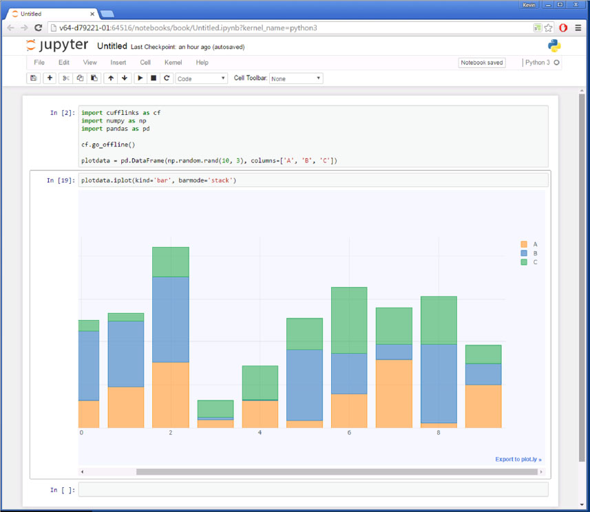
Plotly is another popular plotting package for Python as well as for several other languages. Although you can use the Plotly Python interface directly, it’s easier to plot DataFrames with the additional package named Cufflinks. The Cufflinks package adds an iplot method to DataFrames that works much like the plot method. Note that at the time of this writing, Plotly and Cufflinks were not included in the Anaconda Python distribution, so you might need to install them separately.

In the code in the preceding screenshot, we import Cufflinks and use the go_offline function to indicate to Plotly that the plot is not to be published to the web. We then generate some random data just as in the preceding example. In this case, we use the iplot method on the DataFrame to plot the data.
Just as with the plot method, we can change the type of the plot using the kind parameter. In the following code, you see that we changed the plot to a bar chart with stacking enabled.
For more customized plots, Matplotlib is the preferred tool for most Python programmers. Let’s look at that next.
Creating Graphics with Matplotlib
Although the Matplotlib package is powerful, it does have a bit of a learning curve. We do a simple introduction here, but going further requires some homework. Let’s try to create the same stacked bar chart that we got by using the plot method of DataFrame. That way, we can see what the plot method has to do behind the scenes.

You see in the preceding code that we have to plot each set of bars in the chart individually. We use the row labels of the data on the Y axis and the value of each of the columns (A, B, C) on the X axis. In order to stack them, we must give the starting left point of each subsequent bar in the left keyword parameter. Finally, we set the color of each bar. After we complete the plotting, we adjust the ticks so that the index values are centered on the bars, and we add a legend.
Matplotlib entails more work than does the simple one-liner of the DataFrame plot method. It is easier to use the plot method unless you have specialized requirements.
If you create graphics for the web and want to use an interactive tool, consider using Bokeh. Let’s take a quick look at it in the next section.
Interactive Visualization with Bokeh
Much like Plotly, Bokeh is a Python package for creating interactive visualizations in a web browser. We do a line plot and a bar chart as we did in the other examples. The line chart is fairly straightforward. You can pass a DataFrame into the Line object and display it with the show function.

The creation of a stacked bar chart is quite challenging with the data in the form that we have. You need to restructure it so that all of the values of all columns are in a single column of a DataFrame. The column names must be a value in another column. The reason for this is that the Bokeh bar chart is primarily set up to do groupings and to compute aggregated values. So we need to structure the data so that it works in that model.

Conclusion
If you haven’t used Python much in the past, this coverage might seem like a whirlwind of information. But hopefully you have a good overview of the parts of Python that are used in the rest of this book. As we mentioned previously, there are many Python resources on the web as well as many books on various areas of Python that you might explore.
1 The magic commands are part of IPython. They are not included in standard Python. So they can be used only in the context of an IPython interpreter or a Jupyter notebook.