
9
Linear Regression
Art, like morality, consists of drawing the line somewhere.
Gilbert Keith Chesterton
9.1. Introduction
In the previous section, we discussed the existence of relationships or “correlations” between variables, and the task of discovering these correlations in order to measure the strength of the relationships among several variables. But in most cases, knowing that a relationship exists is not enough; to better analyze this relationship, we have to use “linear regression”.
Linear regression, which we will look at in this chapter, can be used to model the relationships between different variables. Globally, the approach on which this method aims to explain the influence of a set of variables on the results of another variable. In this case, it is called a “dependent variable” because it depends on other variables (independent variables).
Regression is an explanatory method that makes it possible to identify the input variables that have the greatest statistical influence on the result. It is a basic algorithm that any enthusiast of Machine Learning practices must master. This will provide a reliable foundation for learning and mastering other data analysis algorithms.
This is one of the most important and widely used data analysis algorithms. It is used in many applications ranging from forecasting the prices of homes, cars, etc. or the weather, to understanding gene regulation networks, determining tumor types, etc.
In this chapter, you will learn about this algorithm, how it works, and its best practices. This chapter will explain how best to prepare your data when modeling using linear regression. Through case studies and using Python, you’ll learn how to make predictions from data by learning the relationships between the characteristics of your data and continuous value observed responses.
This is an introduction to this method in order to give you enough basic knowledge to use it effectively in the process of modeling for the other kinds of questions you’re likely to encounter while working on Big Data projects.
Let’s examine how to define a regression problem and learn how to apply this algorithm as a predictive model using Python.
Note that we are not going to go into detail about the code: for this we recommend that you refer to specialized work and other information on the subject and that you work through it.
9.2. Linear regression: an advanced analysis algorithm
Linear regression is a data analysis technique used to model the relationship between several variables (independent variables) and an outcome variable (dependent variable).
A linear regression model is a probabilistic model that takes into account the randomness that may affect a particular result. Depending on previously known input values, a linear regression model predicts a value for the dependent (outcome) variable.
This method is mainly used to discover and predict the cause and effect relationships between variables. When you only have one independent variable (input variable), the modeling method is called “simple regression”. However, when you have multiple variables that can explain the result (dependent variable), you must use “multiple regression”.
The use of either of these methods depends mainly on the number of independent variables and, of course, on the relationship between the input variables and the outcome variable. Both simple and multiple linear regression are used to model scenarios for companies or even governments. In the sharing economy context, regression can be used, for example, to:
- – model the price of a house or apartment depending on the square footage, number of rooms, location, etc.;
- – establish or evaluate the current price of a service (rental rules, online assessment notes, etc.);
- – predict the demand for goods and services in the market;
- – understand the different directions and the strength of the relationships between the characteristics of goods and services;
- – predict the characteristics of people interested in goods and services (age, nationality, function, etc.). Who takes a taxi, for example, or requests a particular service, and why?;
- – analyze price determinants in various sharing economy application categories (transport, accommodations, etc.);
- – analyzes future trends (predicting whether the demand for a home will increase, etc.).
Overall, regression analysis is used when the objective is to make predictions about a dependent variable (Y) based on a number of independent variables (predictors) (X). Before diving into the details of this analysis technique, why should it be used and how should it be applied? Let’s see what a regression problem looks like.
9.2.1. How are regression problems identified?
You do not really need to know the basic fundamentals of linear algebra in order to understand a regression problem. In fact, regression takes the overall relationship between dependent and independent variables and creates a continuous function generalizing these relationships (Watts et al. 2016).
In a regression problem, the algorithm aims to predict a real output value. In other words, regression predicts the value on the basis of previous observations (inputs) (Sedkaoui 2018a).
For example, say you want to predict the price of a service you want to offer. You will first collect data on the characteristics of people who are looking for the same service (age, profession, address, etc.), the price of the services already offered by others on a platform, etc. Then you can use that data to build the model that allows you to predict the price of your service.
A regression problem therefore consists of developing a model using historical data to make a prediction about new data for which we have no explanation. The goal is to predict future values based on historical values.
It should be noted that, before starting the modeling phase, three elements in the construction of a regression model must be considered (Sedkaoui 2018b):
- – description: the essential first step before designing a model is describing the phenomenon that will be modelled by determining the question to be answered (see the data analysis process described in Chapter 6);
- – prediction: a model can be used to predict future behavior. It can be used, for example, to identify potential customers who may be interested in a given service (accommodations, etc.);
- – decision-making: tools and forecasting models provide information that may be useful in decision making. Their activities and actions will lead to better results for the company through the “intelligence” provided by the model creation process.
The model therefore provides answers to questions anticipating future behavior and a phenomenon’s previously unknown characteristics to identify specific profiles. How are models built?
9.2.2. The linear regression model
As its name suggests, the linear regression model assumes that there is a linear relationship between the independent variables (X) and the dependent variable (Y). This linear relationship can be expressed mathematically as:
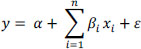
where:
- – y : is the dependent (outcome) variable;
- – xi: are the independent variables (input) (for i = 1, 2, …, n);
- – α : is the value of y when xi is equal to zero;
- – βi: is the change in y based on a unit change in xi;
- – ε : is a random error term representing the fact that there are other variables not taken into account by this model.
The model is therefore a linear equation that combines a specific set of input values to find the solution that best matches the result of this set. This equation assigns a scaling factor to each input value, known as the parameter, which is represented by β. Thus, another factor is added to this equation, called the intercept parameter (α). Any calculation or selection of α and β allows us to obtain an expected result for each input xi.
This model is constructed in order to predict a response (Y) from (X). Constructing a linear regression model involves estimating the values of the parameters, for which α and β are used. For this, we can use several techniques, but ordinary least squares (OLS) is most commonly used to estimate these parameters.
To illustrate how OLS works, imagine that there is only one input variable (X) required to create a model that explains the outcome variable (Y). In this case, we collect n combinations (x, y) that represent the observations obtained, and we analyze them to find the line or curve that is closest to reality or that best explains the relationship between X and Y. The OLS method allows you to find this line by minimizing the sum of squares of the difference between each point and this line (Figure 9.1). In other words, this technique makes it possible to estimate the values of α and β so that the sum indicated in the following equation is minimized:

We should also note that the “Gradient Descent” method is the most commonly used Machine Learning technique. We will not go into the details of how this method works, but you will find an overview of “Gradient Descent” below.
It should be noted here that, when building a model, your goal is to find the model that reflects reality. In other words, one that best describes the studied phenomenon.
In this case, it is worth mentioning that to build such a model, you need to minimize the Loss of information, which refers to the difference between your model, which presents an approximation of the phenomenon, and reality. In other words, the smaller the gap, the closer you are to reality and the better your model.
But how can we reduce this gap? This is what we will discuss in the next section. Before turning to the application of the algorithm, we’ll examine the concept of loss, which is a very important concept in model construction that you need to know to understand linear regression.
9.2.3. Minimizing modeling error
The whole reason for the existence of regression is the process of loss function optimization. This loss may be indicated by the so-called “error”, which refers to the distance between the data and the prediction generated by the model, as shown in Figure 9.1.

Figure 9.1. Difference between model and reality. For a color version of this figure, see www.iste.co.uk/sedkaoui/economy.zip
Determining the best values for parameters α and β will produce the line (the model) that most closely fits the observations. To do this, you need to convert this into a minimization problem in which you seek to minimize the error (loss) between the predicted value and the actual value.
We have chosen to illustrate the loss graphically, because visualization is very useful for evaluating the distance between the observed values and the values calculated by the model. From this figure, we can see that in fact it is the distance between the observation and the line that measures modelling error.
Basically, for each observation, you take the difference between the calculated value (ŷ) and the observed value (y). Then you take the square and finally the sum of squares over all of your observations. Finally, you divide this value by the total number of observations. This short equation provides the Mean Squared Error (MSE) over all observed data points:
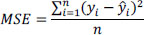
MSE is the most commonly used regression loss function. It shows the sum of the squared distances between your target variable and the predicted values. This is probably the most frequently used quantitative criteria for comparing calculated values and observed values.
But it should be noted that we can prove mathematically that maximizing the probability is equivalent to minimizing the loss function. The goal is to converge on the maximum likelihood function for the phenomenon under consideration, by beginning β from the initial observations.
In this context, we can say that a large part of modelling lies in the optimization methods, that is to say, the methods that seek a maximum or minimum for a given function (Sedkaoui 2018a).
Although linear regression can be applied to a result that represents multiple values, the following discussion considers the case in which the dependent variable represents two values such as true/false or yes/no. Thus, in some cases, it may be necessary to use correlated variables.
To address these problems, the next section of this chapter provides some techniques that we can use in the case of a categorical dependent variable (logistic regression) or if the independent variables are highly correlated.
9.3. Other regression methods
In the linear regression method, as we have previously explained, the results variable is a continuous numeric variable. But if the dependent variable is not numeric and is instead categorical (Yes/No, for example), how can we create a regression model?
In such a case, logistic regression may be used to predict the probability of a result on the basis of a set of input variables.
Thus, in the case of multicollinearity, it may be prudent to impose restrictions on the magnitude of the estimated coefficients. The most popular approaches are the so-called Ridge and Lasso regression methods.
In this section, we will explain these three methods. Let’s begin with logistic regression.
9.3.1. Logistic regression
Logistic regression is a method for analyzing data-sets in which the dependent variable is measured using a dichotomous variable; in other words, there are only two possible results.
This type of regression is used to predict a binary outcome (1/0, Yes/No, True/False) from a set of independent variables. To represent binary/categorical outcomes, we use nominal variables.
This type of regression can be used to determine whether a person will be interested in a particular service (an apartment on Airbnb, an Uber, a ride in a BlaBlaCar, etc.).
The data-set comprises:
- – the dependent (outcome) variable indicating whether the person has rented on Airbnb, requested an Uber, etc. during the previous 6 or 12 months, for example;
- – input variables (independent), such as: age, gender, income, etc.
In this case, we can use the logistic regression model to determine, for example, if a person will request an Uber in the next 6 to 12 months.
This model provides the probability that a person will make a request during that period.
Logistic regression is considered a special case of linear regression when the outcome variable is categorical. In simple terms, this method predicts the probability that an event will occur by fitting the data to a logistic function (logit).
A logistic function f(y), also called a “sigmoid function” , is an S-shaped curve that can take any real number and map it to a value between 0 and 1, as shown in Figure 9.2.
Given that the range varies between 0 and 1, the logistic function f(y) seems to be appropriate for modeling the probability of occurrence for a particular result. As the value of y increases, the probability of the result increases.
After explaining the logistic regression model, we will examine the other models used to address problems of multicollinearity.
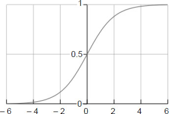
Figure 9.2. The logistics function
9.3.2. Additional regression models: regularized regression
If several input variables are highly correlated, this condition is called “multicollinearity”. Multicollinearity often leads to estimates of parameters of a relatively large absolute magnitude and an inappropriate direction. Where possible, most of these correlated variables should be removed from the model or replaced by a new variable. In this case, we can handle this regression problem by applying particular methods.
9.3.2.1. Ridge regression
This method, which applies a penalty based on the size of the coefficients, is a technique that can be applied to the problem of multicollinearity. When fitting a linear regression model, the goal is to find the values of the parameters that minimize the sum of the squares. In Ridge regression, a penalty term proportional to the sum of the squares of the parameters is added to the residual sum of squares.
9.3.2.2. Lasso regression
Lasso regression (Least Absolute Shrinkage Selector Operator) is a related modeling technique wherein the penalty is proportional to the sum of the absolute values of the parameters.
The only difference from the Ridge regression is that the regularization term is an absolute value. The Lasso method overcomes the disadvantage of the Ridge regression by punishing not only high values of parameter β, but by setting them to zero if they are not relevant. Therefore, we can end up with fewer variables in the model, which is a huge advantage.
After discussing the basics of modelling, linear regression, logistic regression and the Ridge and Lasso extensions, we now turn to action.
9.4. Building your first predictive model: a use case
Having previously discussed the principle of the regression method, let’s now examine how we can build a model and use data. For this, we will use a simple data-set for applying the algorithm to “real” data.
But keep in mind that our goal is far from a simple explanation to help you understand how to build a model for predicting the behavior of Y based on X. Our intent is to illustrate the importance of algorithmic applications in the sharing economy context. Therefore, in this chapter, as in other chapters of this final section, we will use databases from this economy’s businesses, which we have compiled from specific sources.
Since this chapter is focused on regression, we will try, based on the data we retrieve, to model a phenomenon by adapting the linear regression approach. The point here comes down to the execution of a simple model that, hopefully, will help you to better understand the application of this method, by using Python.
Let’s go!
9.4.1. What variables help set a rental price on Airbnb?
Suppose you want to participate in one of the sharing economy’s activities and you have an apartment located in Paris, for example, that you plan to offer for rental to Airbnb customers. For this you must set a price for your apartment.
But how are you going to do this? Quite simply, by adopting a linear regression approach, which will allow you to build a model that explains the price based on certain variables.
You will try to predict the price of your product and define the variables that affect it. In other words, you will identify the variables that are important for setting rent, those that you will need to consider when preparing your apartment listing.
Before starting to create our model, we must clearly understand the goal, define it, and formulate some initial questions that may explain or predict the outcome variable (prices). This will guide the processes of analysis and modelling.
Identifying questions such as “what need are we trying to meet?” or “what variables should be considered?” will guide us to the best model and to the variables that we should considering using. In this context, we should therefore:
- – prepare and clean the data (identify missing data, etc.);
- – explain what we are preparing to present in order to define a way to measure the model’s performance (by identifying potential correlations between different variables, for example);
- – choose a model that includes the variables that are likely to improve the accuracy of the predictive model. In our case, we will choose linear regression.
So, the goal is clear: to model prices for Airbnb apartments in Paris. We want to build our own price suggestion model.
But to create this model, we have to start somewhere. The database used in this specific case was compiled in December 2018 in CSV format (listings.csv), and includes 59,881 observations and 95 variables, accessible to all through the Airbnb1 online platform.
We will analyze this database and build our model – which will allow us to learn many things about your apartment – in three phases:
- – the data preparation phase, which aims to clean the data and select the most significant variables for the model;
- – the exploratory data analysis phase;
- – the modeling phase using linear regression.
But before performing these three phases, we must transform our data set into something that Python can understand. We will therefore import the pandas library, which makes it easy to load CSV files. We will use the following Python libraries:
- – NumPy;
- – matplotlib.pyplot;
- – collections;
- – sklearn;
- – xgboost;
- – math;
- – pprint;
- – preprocessing;
- – LinearRegression;
- – Mean Squared Error;
- – r2_score.
Let’s now move on to the first phase, that of data preparation.
9.4.1.1. Data preparation
The first thing to do in the data analysis process, as we saw in Chapter 6, is to prepare the material that we will use in order to produce good results. Data preparation therefore constitutes the first phase of our analysis. But before taking this step, let’s look at our database for a moment (Figure 9.3).
Now we will clean and remove some variables in this first phase of analysis. The goal is to keep those that are able to provide information to the modeling process.
As the database file contains 95 variables, we removed those that seem useless (like: id, name, host_id, country, etc.) and many more columns containing information about the host, the neighborhood, etc. Obviously, this type of variable will not be useful for this analysis.
All of the retained variables form the linear predictor function, whose parameter estimation consists of formulating a modelling approach using linear regression. From this, we conducted an initial review of 39 independent variables for which 59,881 observations would be used to model the expected value in euros for a night of accommodations in your apartment.
The nature of these variables is therefore both quantitative and qualitative. Quantitative variables contain, for example, the number of comments, certain characteristics such as: latitude/longitude, etc. Qualitative variables include the neighborhood, room_type, etc.

Figure 9.3. Overview of the data-set
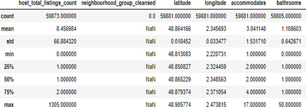
Figure 9.4. Variables with missing values
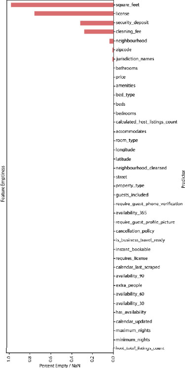
Figure 9.5. The emptiness of the function for all variables. For a color version of this figure, see www.iste.co.uk/sedkaoui/economy.zip
Now that we know our variables, we can proceed with data preparation.
Using the describe function in Python, we can identify the variables with missing values, which we described previously, as shown in Figure 9.4.
We note first that all non-numeric variables are eliminated. Due to the nature of the regression equation, the independent variables (xi) must be continuous. Therefore, we must consider transforming categorical variables into continuous variables.
What about the other categorical variables (qualitative)?
You would like, no doubt, to find out which of the model’s variables are empty. For this, we will use the percent_empty function to allow you to see all the variables and to represent the results graphically (Figure 9.5).
From this figure, we can say that the square_feet variable does not contain any value (almost 100%).
Similarly, the license, security_deposit, and cleaning_fee variables contain missing values at a rate of more than 30%. Therefore, we will remove these variables. There are also other variables that contain missing values, namely: neighborhood, zipcode, and jurisdiction_names, but since the percentage is very small, we can incorporate them into the model.
For the remaining variables, we will eliminate the street variable because we already have information in zipcode, as well as the calendar_updated and calendar_last_scraped variables.
Thus, we can see that certain variables contain the variable “NA”, which we won’t use in the next part of the analysis because they have no value for modeling.
This phase allows us to obtain descriptive statistics for the dependent variable (price) in our model, such as: the mean, standard deviation (std), and the minimum and maximum values, as shown in Table 9.1.
Table 9.1. Descriptive statistics
| Parameter | Value |
| Mean | 110.78 |
| Standard deviation | 230.73 |
| Min | 0 |
| Max | 25,000 |
These statistics, in addition to the graphics, of course, are very useful for understanding the data used. For example, we can say that the average price of apartments in Paris in all the observations is 110.78 euros per night.
Another important point to mention here is that we have a very high maximum value (25,000) compared to the mean. Our work is therefore not finished, and we have to look into this. Is this a false value? If this is the case, how should we handle this problem?
To answer these questions, we will use the sort_values function to pull data from the price variable in descending order.

Figure 9.6. Apartment prices in descending order. For a color version of this figure, see www.iste.co.uk/sedkaoui/economy.zip
The results in Figure 9.6 show that this is not an inconsistency, but only a high proportion of the apartment’s price.
After preparing the data, we will move onto the next stage!
9.4.1.2. Exploratory analysis
After determining the explanatory variables that will be used in the model, it is important to now consider whether each provides completely or partially overlapping information. This is defined in the regression process as “multicollinearity”, which exists when two or more independent variables are highly correlated.
To detect the existence of this type of regression problem, and before proceeding with modelling, the correlations must be analyzed. In other words, for you to better understand this data and to identify interesting trends by building our model, we will examine variables that may be correlated with each other.
It should be noted here that we will mainly use the pandas libraries to browse the exploratory data analysis workflow and to manipulate our data, along with seaborn and matplotlib to draw the necessary graphics.
For this, we used the corr function, and the results are presented in Figure 9.7.

Figure 9.7. Correlation matrix. For a color version of this figure, see www.iste.co.uk/sedkaoui/economy.zip
Figure 9.7 outlines the Pearson correlation coefficient when examined by means of pairwise comparisons.
In this figure, we want to show you how to create a visual graph (data visualization), which will allow us to see the values more clearly. Two colors are used (red and blue) to help us better understand the correlations between the different variables.
The color red represents a negative correlation and the intensity of scaling is dependent on its exact value. The color blue, meanwhile, represents a positive correlation.
By analyzing the correlations, we found some moderately strong (positive or negative) relationships between the different features. The results of the correlation analysis, which varies from positive to negative correlation (see the measurement scale), reveals that there is a clear positive correlation, for example:
- – between availability_60 and availability_90 (0.94);
- – between host_total_listings_count and calculated_host_listings_count (0.88);
- – between accommodates and beds (0.86).
The other variables, however, are only moderately or weakly correlated with each other. So, we decided to delete some and keep others like availability_90 because this variable is weakly correlated with other variables.
Therefore, we’ll only keep the host_total_listings_count variable, etc.
We’ll also eliminate variables with NA results (empty lines or columns in Figure 9.7), which includes: requires_license, has_ availability, and is_business_travel_ready, which will not be useful for our model.
The selection of explanatory (independent) variables is now complete. We finally have a data framework with 20 variables and 58,740 observations (98% of all observations). And we have deleted a total of 75 variables.
Now we have to deal with the characteristics of our dependent variable, “apartment prices” (price). For this, we’ll import the shuffle function, which intermixes the data-set to achieve a series of good results, or model.
Let’s go!
First, it is important to examine the distribution of our dependent variable (price). Figure 9.8 provides us with information about its overall distribution.

Figure 9.8. Price distribution. For a color version of this figure, see www.iste.co.uk/sedkaoui/economy.zip
We see that the prices in this data-set are highly asymmetrical (2.39). In Figure 9.8, we can also see that most of the data points are below 250 (A). We will use a subset of our database, where the price varies from 50 to 250, to remove the very high and low prices. We’ll also transform the target variable to reduce the asymmetry (B).
Now, let’s examine the effects of different variables that have an effect on prices.
In Figure 9.9, you will find box plots for some of the variables in relation to price. They show consistency among variables such as room_type, bed_type, and property_type, which could affect the price of the house or apartment (Figure 9.9).
This figure shows comparative box plots for these variables. We note that there is a price difference between the condition of the room or the apartment in general. Therefore, cleanliness, room type, and bed type are the most expensive options to select at Airbnb apartments in Paris.
Now, let’s look at other available features, such as bedrooms and bathroom. The results show that there is a positive relationship between physical characteristics and prices. This seems reasonable, because the best equipped apartments are undoubtedly the most expensive (Gibbs et al. 2018).
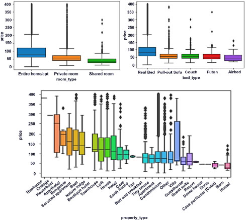
Figure 9.9. Apartment prices as a function of certain characteristics. For a color version of this figure, see www.iste.co.uk/sedkaoui/economy.zip
Figure 9.10 shows the effect of the number of bedrooms and bathrooms on the price per night for Airbnb apartments in Paris. These two features are very important for setting the price, as the correlation coefficient between these two variables confirms (0.62).

Figure 9.10. Price per number of bedrooms/bathrooms. For a color version of this figure, see www.iste.co.uk/sedkaoui/economy.zip
But are bedrooms and bathrooms the only features of an apartment? Of course not! We should also take into account another very important feature that can also influence the price. These are amenities, namely an apartment’s conveniences.
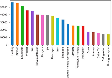
Figure 9.11. Distribution of prices as a function of amenities. For a color version of this figure, see www.iste.co.uk/sedkaoui/economy.zip
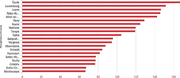
Figure 9.12. The price/neighborhood relationship. For a color version of this figure, see www.iste.co.uk/sedkaoui/economy.zip
The database includes over 65 amenities, and Figure 9.11 shows the 20 most popular features. Heating, basic equipment, kitchen equipment, and television sets are among the most common amenities that Airbnb apartments provide for clients.
The apartment’s location is also an important factor that often has a significant impact on prices. For you to really see how important it is, we have shown price as a function of neighborhood in the following figure. Figure 9.12 shows the location of the apartment is important and that it strongly influences the price.
Before finishing this step and going to the next one, we selected numeric variables and explored them all together. Thus, we have transformed categorical variables into a numeric format. This process converts these variables into a form that can be read by Machine Learning algorithms to achieve a better outcome prediction.
Now that we have finished the exploratory data analysis phase, we can move to modeling.
9.4.1.3. Modeling
Exploratory analysis allowed us to conclude that the overall condition of the apartment affects the price. Other important features you should consider are cleanliness, type of room and bed, square footage, etc. Some additional information, such as access to shops and public transportation, is very useful for setting the apartment price.
In the end, we selected 20 independent variables (Table 9.2) that are the most promising on the basis of the exploratory analysis we performed.
Table 9.2. List of explanatory variables
| Dependent variable | Independent variable | |
| Price | host_total_listings_count | Neighborhood |
| Zipcode | property_type | |
| Latitude | room_type | |
| Longitude | Accommodates | |
| Bathrooms | Bedrooms | |
| Beds | bed_type | |
| Amenities | guests_included | |
| extra_people | availability_365 | |
| maximum_nights | minimum_nights | |
| instant_bookable | calculated_host_listings_count | |
In this step we wanted to manipulate certain characteristics of our dependent variable (price), since they are recovered in price format, and the data contains the thousands separator (“,”) and the “$” symbol. For this, we performed the following operation:
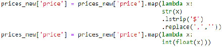
Then we moved on to the modelling step, which involves the evaluation of the model (among those tested) that gives the best results, making it possible to generalize the results to unused data.
Since the objective of this case study is to build a model to predict the prices of Airbnb apartments in Paris, the type of model we are using is a linear regression model. So, we chose to perform a linear regression to account for the various dependencies that may be present in the data.
To resolve the multicollinearity problem between some of the independent variables, we also used Lasso and Ridge regression.
Before turning to the application of the model, it is essential to divide (split) the data into testing sets (train), so as to create a set of unchangeable data for assessing the model’s performance.

Given that:
- – X_train: all predictors in the test data-set (train);
- – Y_train: the target variable in the test;
- – X_test: all predictors for the entire test;
- – Y_test: the target variable in the test set; in our case, it’s price.
In this context, we used sets of variables that were pre-processed and developed in the previous step to perform these operations, using different combinations of variables. Then we adjusted the parameters for each model that was developed; then we selected the model with the greatest available precision.
This optimization process is the final step before reporting results. It makes it possible to find a parameter or a set of robust and powerful parameters using an algorithm for a given problem.
For the Ridge and Lasso regression models, we tested different parameters α (0.001, 0.01, 0.1, 1, 10, 100). The hyperparameters for each model and their validation scores are described in Table 9.3.
Table 9.3. RMSE for different regression models
| Model | Hyperparameter | RMSE |
| Linear regression | By default | 2368.59 |
| Ridge | Alpha = 1.00 | 14.832 |
| Lasso | Alpha = 0.1 | 15.214 |
We can see from the results in Table 9.3 that linear regression does not do a good job of predicting the expected price because our set of variables contains many correlated data points. It was over-adjusted for Airbnb apartments in Paris, which led to horrible RMSE scores.
Thus, we can infer that Ridge regression outperformed Lasso. Ridge regression seems to be best suited for our data, because there is not much difference between the scores of the (train) and (test) data-sets.
We can conclude that the prices of Airbnb apartments in Paris are heavily dependent on available equipment and location. Indeed, most of the variables that have led to price increases are related to equipment and location.
We can apply other algorithms, such as “random forest”, decision tree, etc. to see if these characteristics (amenities/location) are the main factors for predicting the prices of Airbnb apartments in Paris. But we’ll leave that to the next chapter, in which we’ll study these algorithms more thoroughly.
9.5. Conclusion
The key to conducting good data analysis is still mastering the analysis process, from data preparation to the deployment of results, passing through exploration.
Yes! It’s not as easy as it seems, but it’s one of the steps to be followed to achieve the goal.
In this chapter, we used a real-world database to create a predictive model for the prices of Airbnb apartments in Paris. We used a real case study to show you the potential of analytics and the power of data. Furthermore, this example has allowed us to explore our original question concerning which variables influence the price.
The creation of a predictive model for Airbnb prices using regression models provided us with information on the 59,881 observations we analyzed.
The analysis began with the exploration and examination of the data to perform the necessary transformations that will contribute to a better understanding of the problem.
This guided us in the selection of some important characteristics, by determining a correlation between how these characteristics lead to higher or lower prices.
Many of you will now want to, no doubt, make the most of regression and learn how to apply its concepts in areas that interest you. So, what you really need is to practice using other examples, such as Uber, BlaBlaCar, etc.
This will not only allow you to use regression models to predict future trends that you would perhaps not have thought of before, but also to delve deeper into the analytics universe.
TO REMEMBER.– In this chapter, we learned that:
- – linear regression is used to predict a quantitative response Y from predictive variable(s) X; it assumes a linear relationship between X and Y;
- – during the creation of a linear regression model, we:
- - try to find a parameter;
- - try to minimize the error;
- – the use of regression to model Airbnb data allowed us to predict future outcomes;
- – we can use other regression models such as logistic regression (categorical variables) and Ridge and Lasso regression (multicollinearity);
- – although regression analysis is relatively simple to perform using existing software, it is important to be very careful when creating and interpreting a model.
- 1 Available at: http://insideairbnb.com/get-the-data.html.