
11
Cluster Analysis
The Milky Way is nothing more than a mass of innumerable stars planted together in clusters.
Galileo Galilei
11.1. Introduction
In the previous two chapters, we examined the use of supervised learning techniques, regression and classification, to create models using large sets of previously known observations. This means that the class labels were already available in the data-sets.
In this chapter, we’ll explore cluster analysis, or “clustering”. This type of analysis includes a set of unsupervised learning techniques for discovering hidden and unlabeled structures in data.
Clustering aims to seek natural groupings in the data, so that the elements of the same group, or cluster, are more similar than different groups.
Given its exploratory nature, cluster analysis is a fascinating subject, and in this chapter, you will learn the key concepts that can help you organize data into meaningful structures. In this chapter, we’ll address different techniques and algorithms for cluster analysis, namely:
- – learning to search for points of similarity using the k-means algorithm;
- – using a bottom-up approach to build hierarchical classification trees.
This chapter will therefore examine these two algorithms. As you’ll see, the best way to get a good look at the importance of cluster analysis for sharing economy companies is to apply these algorithms to a use case.
We invite you to learn more, in what follows, about this type of unsupervised learning.
11.2. Cluster analysis: general framework
Machine Learning is undoubtedly one of the major assets for addressing both current and future challenges in society. Among the various components of this discipline, we will focus in this chapter on one of the applications that characterizes it: cluster analysis or clustering.
Cluster analysis covers diverse and varied topics and allows for the study of problems associated with different perspectives (Sedkaoui and Khelfaoui 2019). This analysis aims to segment the study population without defining a priori the number of classes or clusters and interpreting the clusters thus created a posteriori.
As part of this analysis, the human does not need to assist the machine in its discovery of the various typologies. No target variable is provided to the algorithm during the learning phase. Clustering consists of grouping a set of observations so that the objects of the same group, called a “cluster”, are more alike in some way compared to other groups or clusters (Sedkaoui 2018b).
In general, this method uses unsupervised techniques to group similar objects. In Machine Learning, unsupervised learning refers to the problem of finding a hidden structure in unlabeled data.
In clustering, no predictions are made, because the different techniques identify the similarities between observations based on the observable attributes and group together similar observations in clusters. Among the most popular clustering methods are the k-means algorithm and hierarchical classification, which we'll cover later in this chapter.
Cluster analysis is considered one of the main tasks of data exploration and a common technique for statistical analysis, and is used in many areas including Machine Learning, pattern recognition, image analysis, information retrieval, bioinformatics, etc.
Finding patterns in data using clustering algorithms seems interesting, but what exactly makes this analysis possible?
11.2.1. Cluster analysis applications
At first glance, one might think that this method is rarely used in real applications. But this is not the case, and in fact there are many applications for clustering algorithms.
We’ve seen them before, when looking at how Amazon (Amazon Web Services) recommends the right products, or how YouTube offers videos based on our expectations, or even how Netflix recommends good films, all by applying the clustering algorithm (Sedkaoui 2018a).
For sharing economy companies, cluster analysis can be used to explore data-sets. For example, a clustering algorithm can divide a set of data containing comments about a particular apartment into sets of positive and negative comments.
Of course, this process will not label the clusters as “positive” or “negative”, but it will produce information that groups comments based on a specific characteristic of these comments.
A common application for clustering in the sharing economy universe is to discover customer segments in a market for a product or service. By understanding which attributes are common to particular groups of customers, marketers can decide which aspects of their campaigns to highlight.
The effectiveness of applying a clustering algorithm can thus enable a significant increase in sales for an ecommerce site or a digital platform.
Sharing economy companies can adopt unsupervised learning to develop services on their platforms. For example, given a group of clients, a cluster analysis algorithm can bundle services and products that may interest its customers based on similarities in one or more other groups.
Another example may involve the discovery of different groups of customers in an online store’s customer base.
Even a chain restaurant can group clients based on menus selected by geographical location, and then change its menus accordingly.
The examples of applications are many and varied in the sharing economy context; we encounter this unsupervised learning algorithm in customer segmentation–a subject of considerable importance in the marketing community– but also in fraud detection, etc.
But how does it work? Good question–we need to look more closely at the details.
11.2.2. The clustering algorithm and the similarity measure
The question now is: how does cluster analysis measure similarity between objects?
In general, cluster algorithms examine a set number of data characteristics and map each data entity onto a corresponding point in a dimensional diagram. These algorithms then combine the similar elements based on their relative proximity in the graph.
The goal is to divide a set of objects, represented by input data:

into a set of disjoint clusters:

to build objects that are similar to each other.
Clustering consists of classifying data into homogeneous groups, called “clusters”, so that the elements of the same class are similar and the elements belonging to two different classes are different. It is therefore necessary to define a similarity measure for any two data points: the distance.
Each element can be defined by the values of its attributes or what we call from a mathematical point of view “a vector”:

The number of elements in this vector is the same for all elements and is called the “vector dimension” (n vector).
Given two vectors V1 and V2. To measure similarity, we need to calculate the distance between these two vectors. Generally, this similarity is defined by the Euclidean distance or by the Manhattan distance (Figure 11.1).

Figure 11.1. Distance calculation
The Euclidean distance presents the distance between two points p and q identified by their coordinates X and Y. We have:

The Manhattan distance, whose name is inspired by the famous New York borough that contains many skyscrapers, calculates the distance as follows:

To calculate the similarity, it is best to choose the Euclidean distance as the metric because it is simpler and more intuitive. Figure 11.2 shows how to group objects based on similarity. The blue segment refers to the distance between the two points. Once we have calculated the distances between each point, the clustering algorithm automatically classifies the nearest or most “similar” points into the same group.
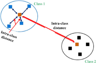
Figure 11.2. The principle of clustering. For a color version of this figure, see www.iste.co.uk/sedkaoui/economy.zip
Clustering algorithms are heavily dependent on the definition of the concept of similarity, which is often specific to the application domain (Sedkaoui 2018b). The principle consists of assigning classes to:
- – minimize the distance between the elements in the same cluster (intra-class distance);
- – maximize the distance between each cluster (inter-class distance).
The goal is to identify groups of similar inputs and to find a representative value for each cluster. You can do this by examining the input data-sets, each of which is a vector in a dimensional space. In this context, two algorithms are frequently used: k-means and hierarchical classification.
In the next section we will discuss the k-means algorithm, which is widely used in the workplace, in detail.
11.3. Grouping similar objects using k-means
Clustering is a technique for searching for groups of similar objects, or objects that are more closely related to each other than objects belonging to other groups. Examples of clustering applications, which we have previously cited from sharing economy companies, can include the grouping of documents, music, and films on various subjects, or of customers with similar interests (bikes etc.) based on purchasing behavior, or of requests for a common service as the basis for a recommendation engine.
One of the simplest and most prevalent cluster analysis algorithms is undoubtedly the k-means method. This algorithm can be defined as an approach for organizing the elements of a collection of data into groups based on similar functionality. Its objective is to partition the set of entries in a way that minimizes the sum of squared distances from each point to the average of its assigned cluster.
For example, say you’re looking to start a service on a digital platform and you want to send a different message to each target audience. First, you must assemble the target population into groups. Individuals in each group will have a degree of similarity based on age, gender, salary, etc. This is what the k-means algorithm can do!
This algorithm will divide all of your entities into groups, with k being the number of groups created. The algorithm refines the different clusters of entities by iteratively calculating the average midpoint or “centroid” mean for each cluster (Sedkaoui 2018b).
The centroids become the focus of iterations, which refine their locations in the graph and reassign data entities to adapt to new locations. This procedure is repeated until the clusters are optimized. This is how this algorithm can help you deal with your problem.
We will now describe this algorithm to show you how it works and how we can determine the average.
11.3.1. The k-means algorithm
As you will see in a moment, the k-means algorithm is extremely easy to implement, and it is also very efficient from the viewpoint of calculations compared to other cluster analysis algorithms, which might explain its popularity. The k-means algorithm belongs to the category of clustering by prototype. We will discuss another type of clustering, hierarchical clustering, later in this chapter.
In real clustering applications, we have no information about the data categories. Thus, the objective is to group similar data-sets, which can be done using the k-means algorithm, as follows:
- – randomly choose k centroids from the group of data points as initial cluster centers;
- – assign each group of data to the nearest centroid;
- – assign the class with the minimum distance;
- – repeat the previous two steps until the cluster assignments no longer change.
K-means is a data analysis technique that identifies k clusters of objects for a given value r of k based on the proximity of the objects to the center of the k groups (MacQueen 1967). The center is the arithmetic average of the attribute vector with n dimensions for each group.
We will now describe this algorithm to show you how it works and how it determines the average.
To illustrate the method, we’ll consider a collection of B objects with n attributes, and we’ll examine the two-dimensional case (n = 2). We chose this case because it is much easier for visualizing the k-means method.
11.3.1.1. Choosing the value of k
The k-means algorithm can find the k clusters. This algorithm will select k points randomly to initially represent each class. In this example, k = 3, and the initial centroids are indicated by red, green, and blue points in Figure 11.3.
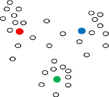
Figure 11.3. Step 1: define the initial points for the centroids. For a color version of this figure, see www.iste.co.uk/sedkaoui/economy.zip
11.3.1.2. Assign each data group to a centroid
The algorithm in this step will calculate the distance between each data point (x, y) and each centroid. It will then assign each point to the nearest centroid. This association defines the first k clusters (k = 3).
11.3.1.3. Assign each point to a class
Here, the algorithm calculates the center of gravity for each cluster defined in the previous step. This center of gravity is the ordered pair of arithmetic averages of the coordinates of the points in the cluster. In this step, a centroid is calculated for each of the k clusters.
11.3.1.4. Update the representatives for each class
We can now recalculate the centroid for each group (the center of gravity). Repeat the process until the algorithm converges. Convergence is reached when the calculated centroids do not change or when the centroid and the attributed points oscillate from one iteration to the next.
Thus, in Figure 11.4, we can identify three clusters:
- – cluster 1: in red;
- – cluster 2: in blue;
- – cluster 3: in green.

Figure 11.4. Step 2: assign each point to the nearest centroid. For a color version of this figure, see www.iste.co.uk/sedkaoui/economy.zip
11.3.2. Determine the number of clusters
The k-means algorithm solves the following problem: “Starting with points and an integer k, the problem consists of dividing the points into k partitions in order to minimize some function.” K-means is the most frequently used clustering algorithm due to its speed compared to other algorithms.
In practice, k does not correspond to the number of clusters that the algorithm will find and where the items are stored, but rather to the number of centers (that is to say, to the center point of the cluster) (Sedkaoui 2018a).
Indeed, a cluster may be represented by a circle with a center point and a radius. We seek to group N points. This algorithm begins with k central points that define the centers of each cluster to which N points will be attributed at the end.
In the first step, the N points are associated with these different centers (initially specified or chosen at random). The next step is to recalculate the centers compared to the average of all points in the cluster.
As we’ve seen from the various steps we’ve already described, we must first find the points associated with the cluster by calculating the distance between the cluster center and these points. Then, the center of the cluster is recalculated until the centers stabilize, indicating that they have reached the optimal values for representing the N starting points.
So, with this algorithm, k clusters can be identified in a data-set, but what value should we select for k? The value of k can be chosen based on a reasonable estimate or a predefined requirement.
At this stage, it is very important to know the value of k, as well as how many clusters are to be defined. So, a measure must be tested to determine a reasonably optimal value for k. The k-means algorithm is easily applied to numerical data, in which the concept of distance can of course be applied.
It should be noted as well that the most frequently used distance for grouping objects is the square of the Euclidean distance, which we have described previously, between two points x and y in an n dimensional space.
Based on this metric of Euclidean distance, we can describe the k-means algorithm as a simple optimization problem, an iterative approach to minimizing the sum of squared errors (intra-cluster) (SSE), sometimes also called the “cluster inertia”:

We can thus deduce that SSE is the sum of the squares of the distances between each point and the nearest centroid. If the points are relatively close to their respective centroid, the sum of the squares of the distances is relatively small.
However, despite its importance, k-means can introduce some limitations related to the following points.
11.3.2.1. Categorical data
As indicated at the end of the previous section, k-means does not support categorical data. In such cases, we use k-modes (Huang 1997), which we haven’t discussed in this chapter, but which is a method commonly used to group categorical data based on the number of differences between the respective components of the attributes.
11.3.2.2. The definition of the number of clusters
It may well be that the data-sets have characteristics that make partitioning into three (3) clusters better than two (2) clusters. We may precede our k-means analysis with a hierarchical classification that will automatically set the best number of classes to select.
In hierarchical classification, each object is initially placed in its own cluster. The objects are then combined with the most similar cluster. This process is repeated until all existing objects are combined into a single cluster.
This method will be discussed in the next section.
11.4. Hierarchical classification
The amount of data available today generates new problems for which traditional methods of analysis do not have adequate answers. Thus, the classical framework of clustering, which consists of assigning one or more classes to an instance, extends to the problems of thousands or even millions of different classes.
With these problems, new avenues for research appear, such as how to reduce the complexity of classification, generally linear as a function of the number of the problem’s classes, which requires a solution when the number of classes becomes too large (Sedkaoui 2018b). Among these solutions, we can cite the hierarchical model.
In this section, we’ll examine hierarchical classification as an alternative to cluster analysis.
11.4.1. The hierarchical model approach
Hierarchical classification creates a hierarchy of clusters. This algorithm will output a hierarchy or a structure that provides more information than a set of unstructured clusters. Hierarchical classification does not require prior specification of the number of classes. The benefits of hierarchical classification are counteracted by lower efficiency.
Hierarchical classification is a classification approach that establishes hierarchies of clusters according to two main approaches. These two main approaches are: agglomerative clustering and divisive clustering:
- – agglomerative: or the bottom-up strategy, wherein each observation begins in its own group, and where pairs of groups are merged upwards in the hierarchy;
- – divisive: or the top-down strategy, in which all observations begin in the same group, and then groups are split recursively in the hierarchy.
In other words, in divisive clustering, we start with a cluster that includes all of our samples, and we iteratively divide it into clusters until each cluster only contains one sample.
On the other hand, agglomerative clustering takes the opposite approach. We start with each sample as an individual cluster and merge pairs of the closest clusters until only one cluster remains.
In order to decide which clusters to merge, a measure of similarity between clusters is introduced. More specifically, this comprises a distance measurement and a linkage. The distance measurement is what we discussed earlier, and a linkage is essentially a function of the distances between the points.
The two standard linkages for hierarchical classification are the single linkage and complete linkage. Single linkage makes it possible to calculate the distances between the most similar members for each pair of clusters and to merge the two clusters with the shortest distance between the most similar members. Complete linkage is similar to single linkage, but instead of comparing the most similar members in each pair of clusters, this method compares the most dissimilar members to perform the merger.
One advantage of this algorithm is that it allows us to draw dendrograms (visualizations of a binary hierarchical classification), which can help in the interpretation of results by creating meaningful taxonomies. Another advantage of this hierarchical approach is that it is not necessary to specify the number of clusters in advance.
11.4.2. Dendrograms
Hierarchical classification provides a tree-like graphical representation called a “dendrogram”. This represents all of the classes created during execution of the algorithm. These classes are grouped, because the iterations are based on the comparison of distances or differences between individuals and/or classes (Sedkaoui 2018b). The size of the dendrogram branches is proportional to the measurement between the grouped objects.
Graphically, we must divide where the branches of the dendrogram are highest; in other words, stop distributing into classes. The graph of the evolution of intra-class inertia as a function of the number of clusters, also aids the graphical selection of the number of clusters or k in the analysis process. This decreases as the number of classes increases.
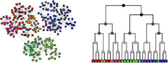
Figure 11.5. K-means versus hierarchical classification. For a color version of this figure, see www.iste.co.uk/sedkaoui/economy.zip
Indeed, they become more homogeneous and decrease in size, and the elements come closer and closer to their cluster centroid. This is actually an abrupt reduction of intra-class inertia based on the number of clusters to be identified.
Different aggregation strategies between two classes A and B can be considered during the construction of the dendrogram. The best known are single linkage, complete linkage, and the Ward criterion.
This criterion considers d as a Euclidean distance, gA and gB as the centroids of the relevant classes, and wA and wB as the respective weights of classes A and B.
The main question that arises in practice is: what criterion should we choose and why?
The answer to this question is summarized in Table 11.1.
Table 11.1. Comparison of different criteria
| Criterion | Use |
| Single linkage | Associated with a minimal tree |
| Complete linkage | Creates compact classes that close arbitrarily |
| Ward Criterion | Minimizes the rise of intra-class inertia |
However, clusters generally have close variances. This is why the most popular choice for users is undoubtedly the Ward criterion. This criterion tends to create rather spherical classes and equal numbers for the same level of the dendrogram. It also is relatively easy to use, even though the distance between elements is non-Euclidean.
Before turning to clustering applications, it should be noted that hierarchical classification is time-consuming. This only applies to incoherent data-sets in terms of the number of elements. The dendrogram is also less readable when this number increases.
Now that you know how these two clustering algorithms work, let’s see how to implement them with Python.
11.5. Discovering hidden structures with clustering algorithms
Clustering maximizes the variance between groups and minimizes the differences within clusters in order to bring the different observations closer together. The database that we will analyze contains 59,740 observations.
In practice, we will perform data classification for different values of k. For each, we will calculate an adjustment. Then we will choose the value of k that leads to the best compromise between a fairly good fit to the data and a reasonable number of parameters to estimate.
The objective is to develop a model that provides a better understanding of all observations. During the analysis process, the clusters will be identified and described. In what follows, we will use the k-means algorithm to separate the data into groups and thus to create clusters with similar values.
11.5.1. Illustration of the classification of prices based on different characteristics using the k-means algorithm
As we saw at the beginning of this chapter, the k-means algorithm is used to group observations near their average. This enables greater efficiency in data categorization.
In this case, the k-means algorithm is used to group characteristics that influence the price of Airbnb apartments in the city of Paris. To run this algorithm, we will use the data-set we used in the previous two chapters.
To better analyze the data using Python, we will import the pandas, NumPy, pyplot and sklearn libraries. We also need the KMeans function from the Scikit Learn library. We will load it from sklearn’s cluster sub-module. Once the data is put into the right format, that is to say into a DataFrame, training the k-means algorithm can be facilitated using the Scikit Learn library.
Our goal is to model the price for the different characteristics using the k-means algorithm. To build our model, we need a way to effectively project the price based on a set of predetermined parameters; therefore, we have chosen to apply this algorithm to identical neighborhoods and listings with similar attributes.
This will ensure that the clusters result from properties that are as similar as possible, so that differences in attributes are the only factor affecting prices and so that we can determine their influence on the price.
The aim is to exploit data on Airbnb prices in Paris. The results of the process will generate useful knowledge for price comparisons. First, we will normalize the data with Minimax scaling provided by sklearn to allow the k-means algorithm to interpret the data correctly.
Figure 11.6 shows the scatter plot for our data.

Figure 11.6. Distribution of observations
Figure 11.6 shows the membership of each observation in the different clusters. However, the results are not very telling, and visually, we can say that three or four groups have formed.
This is the goal of using the k-means algorithm: separating these observations into different groups. Before actually running the algorithm, we must first generate an “Elbow” curve to determine the number of clusters we need for our analysis. The idea behind the “Elbow” method is to find the number of clusters for which the imbalance between the clusters increases most rapidly.
11.5.2. Identify the number of clusters k
This method evaluates the percentage of the variance explained by the number of clusters. Its aim is to separate the observations into different groups. We do this in order to rank the apartments with different pricing models into distinct groups. It is therefore appropriate to choose a number of clu ters such that one additional cluster does not provide a better model.
Specifically, if one plots the percentage of variance explained by the clusters compared to the number of clusters, the first clusters will explain most of the variance. But at some point, the marginal gain of information will drop, creating an angle in the graph. The number of clusters is selected at this point, hence the “elbow criterion”.
This elbow cannot always be unambiguously identified. The percentage of variance explained is the ratio of the intergroup variance to the total variance, also called the “F test”. A slight variation on this method draws the intra-group variance curve. To set the number of clusters k in the data-set, we will use the “elbow” curve. The elbow method takes into account the percentage of variance explained by the number of clusters: one must choose this number such that adding another cluster does not provide a better data model. Generally, the number of clusters equals the value of the x-axis at the point that is the corner of the elbow, which we described in Box 11.3 (the line often resembles an elbow).
Figure 11.7 shows that the score, or the percentage of variance explained by the clusters, stabilizes at three clusters. That's what we’ll include in the k-means analysis.

Figure 11.7. Determination of the number of clusters using the elbow method. For a color version of this figure, see www.iste.co.uk/sedkaoui/economy.zip
This implies that the addition of several clusters does not explain much additional variance in our variable. Therefore, since we were able to identify the optimal number of clusters (k = 3) using the “elbow” curve, we’ll set n_clusters to three clusters.
Once the appropriate number of clusters has been identified, principal component analysis (PCA) can be undertaken to convert data that is too scattered into a set of linear combinations that is easier to interpret.
Now we can run the k-means algorithm. We simply have to instantiate an object of the KMeans class and tell it how many clusters we want to create. Thereafter, we will call the fit() method to compute the clusters. Figure 11.8 shows the membership of each observation by class:
- – cluster 1: observations with a Class 0 in blue;
- – cluster 2: observations with a Class 1 in red;
- – cluster 3: observations with a Class 2 in green.

Figure 11.8. The three clusters. For a color version of this figure, see www.iste.co.uk/sedkaoui/economy.zip
The application of the k-means algorithm has allowed us to divide data-sets into groups based on their characteristics, without needing to know their corresponding labels (y variable).
Using this data led us to better understand the context of our main question. The process of analysis that we carried out in this part’s three chapters has allowed us to interpret the results and to easily identify the most important predictors for setting price.
For each kind of analysis question, a specific group of methods called algorithms can be applied. These algorithms present a real opportunity for change. They make our programs smarter by making it possible for them to automatically learn from the data we provide.
The purpose of this example and of all of the examples we have shown in this part is to demonstrate how you can read and understand your data, apply tools and methods, and visualize your results. The goal is to help you learn to apply the different techniques that we can use to analyze large amounts of data.
With the various examples illustrated in this last part, you can see and understand how data analysis can generate additional knowledge and how it transforms ideas into business opportunities. Big Data analytics has revolutionized business by merging the immensity of big data to draw observations and unique deductions, never before imagined, to better predict the next step to be taken.
11.6. Conclusion
This chapter provided a detailed explanation of cluster analysis. It helped you learn about two different cluster analysis algorithms that can be applied to find hidden structures in data-sets. To demonstrate them in practice, we used a sample database.
In this chapter, you learned how to use the k-means algorithm to group similar observations using the Python programming language. The latter is easy to use. Now, it’s your turn to take up other examples, test a number of different clusters, and see what groups emerge.
TO REMEMBER.–
Overall, what you need to consider when using a clustering approach is summarized in the following points:
- – cluster analysis is an unsupervised learning method;
- – this method groups similar objects based on their attributes;
- – the most frequently used clustering algorithm is the k-means algorithm. To ensure proper implementation, it is important to:
- -properly adjust the attribute values;
- -ensure that the distance between the assigned values is significant;
- -set the number of groups k so that the SSE is reasonably minimized;
- – if k-means does not appear to be an appropriate classification technique for a given set of data, alternative techniques such as hierarchical classification should be considered.