Ecology is an area where evaluation decision problems are frequent, visible, and have wide social impact because they directly or indirectly affect all population. Many human agricultural, industrial, and service activities create different forms of waste and then use environment as a waste sink. Natural systems recycle their waste. Economies are not natural recyclers; when forced, they try to recycle a fraction of waste, but environments are the final repositories of remaining waste products. In addition, even if waste is sufficiently recycled and/or assimilated by environment, the growing human presence creates development and transport activities that cause environmental problems, reducing the natural habitat for fish, wildlife, and plants. That creates a number of delicate decision problems, as well as increasing interest in soft computing techniques for solving such problems [MUN94, VAN04, PAS12, REB14]. LSP is one soft computing decision method that has been successfully used in that context [ALL11, REB16, MES18]. In this chapter, we show the use of LSP criteria for evaluation, comparison, and selection of multispecies habitat mitigation projects.

4.4.1 Multi‐Species Compensatory Mitigation Projects

The first step in the development of LSP criteria is to define a stakeholder. In the case of criteria related to clean air, clean water, global warming, and preserving other species that exist on this planet, it might be possible to claim that the stakeholder is everybody. This is the reason why ecological problems are under governmental regulation: the Endangered Species Act of 1973 [ESA73, WIK16] is used in the United States to protect endangered species from extinction as a consequence of population growth, economic growth, and development. The goal to “halt and reverse the trend towards species extinction” is regularly supported by environmental laws, international treaties [ESA73], and governmental agencies like the United States Fish and Wildlife Service (FWS) and the National Oceanic and Atmospheric Administration (NOAA). In addition, there are nongovernmental organizations devoted to many forms of conservation and environmental protection, such as The Conservation Fund (TCF) [TCF16a].

In this chapter, we describe methodology developed in the context of the TCF strategic conservation planning activity and strategic mitigation for pipelines [TCF16b]. More precisely, we present a family of soft computing decision models used in strategic multispecies habitat mitigation projects [TCF10, DUJ11, ALL11, MES18]. The goal of such projects is to reduce harmful effects on wildlife caused by major energy and/or infrastructure development projects. We present the multispecies habitat mitigation goals and related evaluation decision problems, the selection of soft computing decision models, and the development of the necessary decision support software. Our LSP approach is applicable in all compensatory mitigation projects that are undertaken to compensate wildlife‐related negative effects of various development projects. We present a case study of soft computing decision models for selecting compensatory mitigation projects related to the 15,500‐mile‐long natural gas pipeline network going through 14 states from the Gulf of Mexico to the New York state, operated by NiSource [FWS16c] (before the Columbia Pipeline Group separation and Trans Canada acquisition of the Columbia Pipeline Group).

All major energy and infrastructure development projects cause harmful effects on wildlife habitat and the need for compensatory mitigation projects. That holds for fuel pipelines, wind turbine farms, traditional power plants, and transmission lines, road and rail networks, and others. Such projects may critically impact various threatened species or their habitat.

According to the Endangered Species Act and its amendments [WIK16], lawful development activities require an incidental take permit [FWS16b] issued by the FWS [FWS16a]. The incidental take permit holders provide a Habitat Conservation Plan [TCF16, FWS16c] and secure funding for a plan that minimizes and mitigates harm to the impacted species. In the case of the analyzed natural gas transmission and storage operation, the mitigation projects are related to the 15,500‐mile‐long network of natural gas pipelines that affect the following species: Indiana Bat, Madison Cave Isopod, Nashville Crayfish, Bog Turtle, Clubshell, Fanshell, Northern Riffleshell, Sheepnose, and James Spinymussel [FWS16c]. The implementation of the NiSource Multi‐Species Habitat Conservation Plan (MSHCP) [COL15] is based on the ecological expertise of TCF [TCF16a, TCF16b, MES18], and uses the LSP decision support methodology and corresponding software [TCF16].

Each MSHCP mitigation project includes evaluation of alternatives (candidate species habitat areas), and selection of the most suitable alternative that satisfies the take species habitat mitigation requirements and provides other conservation benefits. Each mitigation project evaluates competitive areas that can be acquired and used primarily or exclusively for conservation of endangered species. Consequently, stakeholders and decision makers (NiSource, TCF, FWS, and state and local governments) must develop criteria that evaluate the overall level of satisfaction of MSHCP conservation requirements, taking simultaneously into account ecological benefits and financial constraints. The ultimate goal of the decision process is to develop solutions that offset the gas pipeline impacts, and offer maximum ecosystem benefits per habitat mitigation dollar.

The criteria for evaluation, comparison, and selection of competitive species habitats consist of a number of requirements that are considered mandatory and a number of requirements that are desired or optional. Such relationships can be modeled using the partial absorption function. Some of requirements must be simultaneously satisfied and need modeling with hard or soft partial conjunction. Other requirements may replace each other, and in such cases we need soft or hard partial disjunction.

Financial aspects of evaluated projects are very important and must be properly aggregated with ecological (nonfinancial) suitability scores to create an overall ranking of competitive mitigation solutions. This chapter exemplifies all major steps of LSP decision methodology in a way that is applicable in a variety of ecological mitigation decision problems. We also use this chapter to exemplify the role of sensitivity analysis in the process of creating LSP criteria.

4.4.2 A Generic LSP Attribute Tree for Evaluation of Habitat Mitigation Projects

The first step in the development of an LSP criterion consists of specifying the attribute tree. The tree must include all attributes that affect the ability of an evaluated area to satisfy MSHCP mitigation requirements for specific species. Some attributes represent mandatory requirements, and in such cases the logic properties of the evaluation criterion must be adjusted so that an MSHCP project is rejected if any of mandatory requirements is not satisfied. Other attributes represent nonmandatory requirements that are desirable and contribute to the suitability of the evaluated MSHCP project. However, if nonmandatory requirements are not satisfied, that will not automatically disqualify the evaluated project.

Our approach is based on a generic evaluation criterion that defines the structure of all MSHCP decision criteria and the corresponding aggregation logic. The generic criterion holds for the whole family of MSHCP projects and can be easily customized for each individual species taking into account specific ecologic requirements that a suitable species habitat must satisfy.

The proposed generic attribute tree, adapted for freshwater mussels, is shown in Fig. 4.4.1. The four top levels of decomposition are generic, i.e., they can be used in almost all mitigation projects. Further decomposition is specific for selected species.

The generic tree consists of two main attribute groups: the take species habitat mitigation requirements (#11) and other conservation goals and benefits (#12). The group #11 should be subsequently adjusted for each specific species. The group #12 includes requirements that are common for the majority of mitigation projects.

The most important subgroup of attributes includes 14 mandatory requirements inside the group #111. These attributes are grouped in five subgroups (denoted #1111 to #1115). Most of the attributes are composite inputs that need a domain expert evaluation. The habitat mitigation requirements also include seven desired and optional requirements that form the group #112. They evaluate the likelihood of protection in perpetuity and the protection of other listed species. These components are not mandatory, but they are certainly very desirable, and their absence should cause significant penalty for evaluated MSHCP projects.

In developing the attribute tree, it is also important to consider general strategic goals and benefits that form the group #12. This group includes six attributes that are used to evaluate whether the analyzed MSHCP projects provide other benefits, such as support for green infrastructure, support for other plans, and human benefits. The requirements in this group are not mandatory. Thus, the proposed generic tree is used to develop 27 elementary input attributes: 14 of them are mandatory and 13 of them are nonmandatory. These attributes should reflect the requirements that are nonredundant (independent of each other) and complete (no missing relevant attributes).

The presented generic tree creates the need for 27 elementary criteria. Some of these attribute criteria are compound and depend on multiple elementary input components. In such cases, there are two options. The first option is to continue decomposing the attribute tree until we reach all elementary inputs and further decomposition becomes impossible (in such cases, the elementary criteria are very simple). The second option is to create scoring attribute criteria where we assign scores to existing elementary inputs and then create the elementary criterion that evaluates the resulting total score. This technique is exemplified in the next section.

4.4.3 Attribute Criteria and the Logic Aggregation Structure

For each elementary input attribute we have to develop a justifiable elementary criterion. The criteria are different for various species and a small sample of typical elementary attribute criteria is shown in Table 4.4.1. The criterion #1111 is classified as the normalized‐variable continuous absolute criterion. The criterion #11131 is an example of the point‐additive criterion, which uses a simple scoring and then evaluates the total score. The criterion #11132 uses direct preference assessment based on a simple five‐level rating scale, and the last two elementary attribute criteria are discrete.

The next step is to develop a generic multi‐species logic aggregation structure. The basic idea is shown in Fig. 4.4.2 and then refined in Fig. 4.4.3. In Fig. 4.4.2 we show the concept of aggregation of the three basic groups of attributes: #111, #112, and #12. The Take Species Habitat Mitigation Requirements (#11) consist of two groups of attributes: mandatory (#111) and non‐mandatory/optional (#112). In that way it is easy to assign each attribute to one of these groups. The aggregation is then performed using a conjunctive partial absorption aggregator. The result of this aggregation (the suitability degree denoted #11) has the mandatory status with respect to the non‐mandatory #12 (Other Conservation Goals and Benefits). Therefore, we aggregate #11 and #12 using another conjunctive partial absorption. The resulting compound aggregator is a nested partial absorption with one mandatory and two optional inputs that should approximately have the same impact on the overall suitability #1 (this is verified in the next section).

The adjustment of CPA parameters is based on selection of desired penalty (average decrease of output suitability caused by the zero optional input) and reward (average increase of output suitability caused by the maximum optional input). The desired penalty and reward values are shown in Fig. 4.4.3 (P25/R20 denotes an average penalty of 25% and an average reward of 20%).

All other aggregators in Fig. 4.4.6 are various forms of GCD, i.e., either a partial conjunction or a partial disjunction. In the case of #1112, #1113, and #1114 we use the hard partial conjunction aggregator C‐+, which is similar to the geometric mean. According to the canonical increasing partial conjunction form the aggregator #111 is also a hard partial conjunction but significantly stronger.

The aggregator #1121 is also hard, regardless its belonging to the group of optional aggregators. This is based on opinion that #1121 (protection in perpetuity) cannot be achieved if any of the five necessary inputs is missing. On the other hand, the aggregator #1122 is disjunctive because the protection of other species can be achieved by any of the two alternative inputs. Similarly, the aggregator #122 is also disjunctive because any of the three alternative plans can sufficiently contribute to the planning goals.

The logic aggregation structure shown in Fig. 4.4.3 is an initial generic solution. We assume that in practical use of the LSP method the criterion will be tuned and altered to generate results that are conformant with stakeholder’s expectations. LSP criteria are expected to model human perceptions, and therefore the results of evaluation must not be significantly different from evaluator expectations. To occurrence of significant differences is sufficient to justify modification of the criterion function.

One of methods to test and verify the behavior of an aggregation structure before it is actually used in practice is to perform a sensitivity analysis. A typical sensitivity analysis is presented in the next section.

4.4.4 Sensitivity Analysis

A detailed suitability aggregation structure shown in Fig. 4.4.3 includes weights (the relative importance of all inputs), aggregation operators, and penalty/reward pairs (denoted P < percent penalty>/R < percent reward>). The weights and aggregation operators are selected to reflect the needs of MSHCP projects. To verify quantitative properties of the aggregation structure we use a sensitivity analysis, where we adjust all input suitability scores to have the same default value s, and then investigate the variations of output suitability caused by changing a single input or subsystem suitability in the range from 0 to 1 (or 0 to 100%). Assuming the default suitability s = 75%, the effects of changing subsystem suitability scores are shown in Fig. 4.4.4. The lowest curve shows the component that causes the highest impact, and that is the subsystems #11 (take species habitat mitigation requirements). The second highest impact is caused by the mandatory habitat requirements subsystem (#111), followed by its components. The optional inputs (#112 and #12) have almost identical impact. All mandatory component curves start from the origin, and all nonmandatory component curves show lower impact and start from positive values. If the default suitability is positive the sensitivity curves are always strictly increasing.

In addition to sensitivity curves it is useful to define sensitivity coefficients that define the properties of sensitivity curves. Suppose that we use the default suitability . So, all inputs are s and due to idempotency the output is also s. The overall effects of changing an input (or subsystem) suitability x_i that affects an output suitability f(x_i) can be characterized using the limit values , , and , . 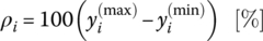We express sensitivity properties using the following basic indicators that are all expressed as percentages:

• Suitability increment:
• Suitability decrement:
• Absolute influence range:
• Conjunctive coefficient of impact:

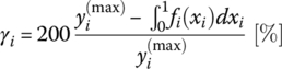
Sensitivity coefficients reflect various aspects of the overall importance of input attributes and their subsystems. The suitability increment shows what improvement of the output suitability can be obtained if the input suitability increases from s to the maximum value (1 or 100%). The suitability decrement shows what worsening of the output suitability would occur if the input suitability decreases from s to the minimum value 0. For all mandatory requirements, . The absolute influence range is the sum of the suitability increment and the suitability decrement. The criterion shown in Fig. 4.4.3 is predominantly conjunctive and the sensitivity curves in Fig. 4.4.4 are concave. For concave sensitivity curves the impact of analyzed input x_i is high if the mean value of the output suitability function f(x_i) is low (no hypersensitivity). This property is characterized using the conjunctive coefficient of impact defined in Section 3.7.1. The use of sensitivity coefficients for ranking of all subsystems of the MSHCP criterion according to the decreasing influence range is shown in Table 4.4.2. In this case, the ranking by decreasing range gives similar results as the ranking according to the decreasing impact. Not surprisingly, the impact of subsystems varies in a wide range and the highest impact comes from subsystems in the group #111. As expected, the impacts of optional subsystems #112 and #12 are almost the same.

A complete sensitivity analysis is usually performed also for all elementary input attributes. The goal is to verify that the ranking of sensitivity coefficients is consistent with evaluator’s expectations. This analysis of MSHCP input attributes is presented in Fig. 4.4.5 and Table 4.4.3. Of course, the impacts of individual inputs are generally less than the impacts of subsystems. The most important mandatory inputs are #1111, #1115, and #11142, and the most important nonmandatory inputs are #121 and #11212. The ranking of input attributes according to sensitivity coefficients is a simple technique for verification of suitability aggregation properties, and it can be performed for various values of default suitability, including those that may be different for each input.

The sensitivity Table 4.4.3 also shows inputs that have a very small impact. This is a frequent in cases where the number of inputs is large. There are three possible actions in response to inputs that have very small impact: (1) to keep them expecting that they contribute to the completeness and precision of the criterion function, and in some cases to force vendors to take them seriously into account, regardless of their low impact; (2) to remove them from evaluation as insignificant, because they increase the cost of evaluation and have low contribution to the evaluation results; and (3) to consider the low impact as a reason to modify the criterion function in order to increase the impact of selected inputs.

4.4.5 Logic Refining of the Aggregation Structure

Elementary criteria for ecological problems are regularly rather complex and include composite indicators. For example, the criterion #11141 (Known & Potential Host Fish) is evaluated as Crit(#11141) = {(0,0), (4,100)} where the values 0–4 are interpreted as follows:

• 4 = Abundant population of multiple known host fish + high fish IBI score
• 3 = Abundant population of at least two known host fish + high fish IBI score
• 2 = No known host fish + high IBI score
• 1 = No known host fish + medium IBI score
• 0 = No known host fish + low IBI score

Host fish are necessary for reproductive process of mussels, and if known host fish are present, that is a sufficient prerequisite for the suitability of evaluated site. However, for some mussel species, the host fish are not known. In such cases, it is possible to use the IBI score (Index of Biotic Integrity [KAR81], a composite index based on biological attributes of an aquatic community) as a proxy for the likely presence of host fish, both known and unknown. Therefore, the abundance of known host fish is a sufficient requirement, the high IBI score is a desired attribute, and the criterion #11141 can be composed as a disjunctive partial absorption of two subcriteria: #111411 Number of Known Host Fish, and #111412 The IBI Score. Assuming 12 ≤ IBI ≤ 60, the appropriate elementary criteria are:

• Crit(#111411) = {(0, 0), (1, 40), (3, 100)}
  • 0 = No known host fish
  • 1 = Abundant population of one known host fish
  • 2 = Abundant population of two known host fish
  • 3 = Abundant population of more than two known host fish;
• Crit(#111412) = {(15, 0), (55, 100)}.

If we want to attain a penalty of 25% and a reward of 50% then the corresponding DPA aggregator and its sensitivity functions are shown in Fig. 4.4.6.

4.4.6 Cost/Suitability Analysis

The cost/suitability analysis provides final results of evaluation and comparison of competitive projects. It combines the analysis of relative suitability (a given competitor suitability score divided by the best competitor suitability score) and affordability (lowest cost divided by a given competitor cost). The goal is to find projects that simultaneously offer high suitability and high affordability.

For M competitive MSHCP projects the LSP criterion function generates the overall suitability scores . The overall suitability scores are computed from strictly nonfinancial input attributes. All competitive projects must provide the overall suitability above the minimum suitability threshold value, which is usually selected from 67% to 75%. All projects that offer the overall suitability below the accepted threshold value are rejected. For projects that are above the minimum suitability threshold we compute the following relative overall suitability:

For each competitive MSHCP project, it is necessary to perform a detailed financial analysis that generates the net present value of all cash flows (both expenses and earnings). This strictly financial analysis generates the overall cost indicators . We assume that the overall cost indicators must be below a selected maximum cost threshold value, and that projects that are above the maximum cost must be rejected. For projects that are below the maximum cost threshold we compute the following relative affordability indicator:

In the majority of practical cases the decision makers are interested to simultaneously attain a high suitability and a high affordability. In a general case, the relative importance of high suitability () is not the same as the relative importance of high affordability (). In some cases it is more important to find an affordable solution, while in other cases it might be more important to attain high suitability. In all cases, .

Now, we are ready to compute the overall values of all MSHCP projects as a logic aggregate L of relative suitability and relative affordability: . The logic aggregator L can be selected either as a generalized conjunction/disjunction or a partial absorption. The most frequently used aggregator is the partial conjunction which can be implemented as a weighted power mean:

The highest value denotes the winning competitor. Consequently, the winning competitor offers simultaneously high suitability and high affordability. In a frequent special case, we can be satisfied with the andness of 67%, and compute the overall value simply as a weighted geometric mean (r = 0):

The overall values V₁, …, V_M are usually computed for all combinations of the weights of suitability and affordability. Then we can see in what range of relative importance of suitability/affordability the winner dominates other competitors. If the dominance is shown for a wide range of weight combinations, then the winner can be selected with high confidence.

4.4.7 MSHCP Software Support

The MSHCP projects are distributed in 14 states, and several evaluation teams may perform the evaluation process simultaneously. To provide centralized support over the Internet and simultaneous access to LSP criteria, the necessary software is developed as a web application called the LSPweb [SEA16]. The overall structure and functionality of the LSPweb system are shown in Fig. 4.4.7.

LSPweb supports five types of users: evaluator, analyst, administrator, and two system users: root and service. Evaluators can define competitive systems and evaluate those using available LSP criteria. Analysts can customize existing LSP criteria (change all parameters) and use modified criteria for evaluation and comparison of competitive systems. Administrators and system accounts (root and service) are authorized to develop evaluation criteria: they can upload new criteria, open and close user accounts, and perform evaluation. Analysts and evaluators are primarily engaged in providing input for the evaluation process and in interpreting and distributing evaluation results.