3
Transport Pooling: Moving Toward Green Distribution
Supply chain pooling is a powerful strategy used to improve the profits and performance of the supply chain. From this perspective, the pooling of shipments has been highlighted and recently studied in several publications. In this context, this chapter attempts to, first, present a general framework for logistical sharing and collaboration and, second, to present a review of the literature in order to follow how these concepts are applied. Subsequently, in the case of distribution in urban and interurban environments, a conceptual framework modeling transport pooling is presented through various scenarios. Finally, we end with an analysis of the proposed scenarios in terms of minimizing the distances traveled and greenhouse gas (GHG) emissions. Consequently, this work allows those people who make use of pooling to choose the most appropriate scenario while pooling resources in order to reduce GHG emissions.
3.1. Introduction
Some logistics activities contribute to congestion, pollution, and wasting of resources. These activities can affect delivery efficiency, mobility, the environment, and human health. This explains the need to develop other strategies in order to create new and more efficient logistics systems such as collaborative logistics. In this case, the shared supply chain is proving to be a useful choice for producers and logistics service providers to improve their economic and environmental performances.
In addition to the traditional objectives of efficiency and control of the supply chain, there are now challenges in terms of CSR (corporate social responsibility) and sustainable development (Chay et al. 2013). To achieve these objectives, entrepreneurs must move toward new inter-organizational configurations, such as logistics pooling, in order to optimize their pooled material resources (warehouses and means of transport) through the appropriate selection of a scenario that minimizes transport and storage costs in addition to the volume of GHG emissions. In order to consolidate the successful pooling of transport, interested parties should share and exchange data and information to facilitate the implementation of this concept (Lundqvist 2018).
In order to improve economic performance while maintaining social and environmental objectives, different forms and approaches to logistics pooling have been studied in several publications, such as collaborative urban transportation (Cleophas et al. 2019), collaborative transportation management (Okdinawati et al. 2015), collaborative transport planning (Wang and Kopfer 2014), collaborative transport between terminals (Gharehgozli et al. 2017), pooled transport for children with disabilities (Tellez et al. 2016), pooling of last-mile delivery (Liakos and Delis 2015), collaborative air traffic flow management (Murça 2018), and collaborative intermodal transport (Liu et al. 2019).
Transport pooling allows partners to benefit from several advantages that lead to green and sustainable transport, integrating sustainable development objectives (Moutaoukil et al. 2013). At the economic level, we can mention the following: the lowering of logistical costs, carbon taxes, and fuel costs (Guajardo and Rönnqvist 2016; Wang et al. 2017). At the ecological level, it is worth mentioning the following: the simultaneous lowering of GHG emissions, noise, the exploitation of natural resources (energy), the encouragement of recycling, and waste processing (Alvarez et al. 2018; Niu and Li 2019; Ntziachristos et al. 2016; Senkel et al. 2013). At the societal level, we can consider the following: the expectations of various stakeholders, establishing a culture of sharing (Wang et al. 2018), minimizing stress for drivers – less congestion (Gonzalez-Feliu and Battaia 2017; Hensher 2018) – and saving time (Ghaderi et al. 2016; Moutaoukil et al. 2015).
In this context, a literature review will be presented to highlight the techniques of collaboration, pooling, and resource sharing, in addition to their benefits for goods-producing companies. Furthermore, a suggestion of seven scenarios for pooling between a set of three companies is discussed. This is done in the urban and interurban distribution phases in order to optimize resources and minimize the distances traveled. As a result, we achieve reductions in transportation costs, congestion, and GHG emissions. In addition, the study continues through the analysis of the presented scenarios in order to choose the optimal path by showing the challenges and opportunities of this pooling.
3.2. Concepts of collaborative logistics
3.2.1. Definitions and issues
The definition of collaborative logistics is difficult to define, given that it differs from one case to another. According to Cao and Zhang (2010), supply chain collaboration refers to the ability of two or more autonomous companies to work effectively together, plan, and execute supply chain operations in order to achieve common objectives. In addition, Moutaoukil et al. (2012) added that pooling is mainly about bringing together efforts to achieve a mutual objective. Thus, independent companies work together to reduce their operating costs and increase their revenues. On the other hand, Moharana et al. (2012) have stipulated that collaboration is a common interactive process that translates into joint decisions and activities, and their joint implementation can be considered as a team effort.
Rakotonarivo et al. (2009) identified four main stages of collaboration: transactional, informational, decision-making, and strategic. In addition, Rajaaa and Ibnoulkatib (2019) have identified four urban logistics issues:
- – functional issues: planning cities to meet traffic needs;
- – economic issues: increasing the size of the market;
- – urban issues: movement of goods in the city and location of these platforms;
- – environmental issues: corporate social responsibility in terms of environmental protection.
However, Chanut and Paché (2013) added that societal issues are also important for preserving the living conditions of future generations, preventing them from being faced with a hostile, polluted, and vehicle-saturated environment. In this social perspective of the sustainability of urban distribution, Wang et al. (2018) proposed a prototype platform for the integration of collaborative and social urban distribution, the objective of which is flexible coordination between the operators described in the crowdsourcing and sharing economy. They stipulate that this open integrated platform gives participants (customers, vendors, suppliers, logistics service providers, and the general public) several advantages. In general, collaboration can be applied in terms of the design (Gonzalez-Feliu et al. 2013), planning and execution of work (Tornberg and Odhage 2018), decisions (Perboli et al. 2016), research and development (Bustinza et al. 2019), risk management (Chen et al. 2013), and so on. It reduces the cost of transport and storage, in addition to allowing significant economic gains. Collaboration thus allows companies to be agile and resilient (Camarinha-Matos 2014).
3.2.2. Forms of logistical collaboration
Companies are currently seeking to create synergies with other organizations and create value chains through horizontal and/or vertical collaboration with logistics partners.
3.2.2.1. Horizontal collaboration
In logistics, horizontal collaboration consists of a collaboration between operators at the same level (between suppliers, manufacturers, distributors, etc.) in a supply network. Vanovermeire et al. (2013) declared that horizontal collaboration can be defined as the grouping of transport companies which operate at the same level of the supply chain, and which have similar or complementary transport needs. It is also a collaboration between a group of stakeholders from different supply chains, acting at the same levels and with similar needs (Gonzalez-Feliu et al. 2013).
According to McKinnon and Edwards (2010), horizontal collaboration overcomes financial and commercial barriers and benefits society by reducing the number of vehicles and, therefore, CO2 emissions and congestion. It also reduces prices due to bulk purchasing, reduces supply risks, reduces administrative costs due to centralized purchasing activities, and also reduces inventory, transport, and logistics costs and facilities. All these benefits are achieved through a rationalization of the use of equipment and better sharing of human labor and information (Bahinipati et al. 2009).
3.2.2.2. Vertical collaboration
Vertical collaboration occurs between partners operating in different levels of the logistics network, where the benefits of collaboration include lower supply costs due to the synchronization effect through information sharing (Moutaoukil et al. 2012). In this regard, Fernandez et al. (2016) have stated that vertical collaboration is proposed when shippers and customers collaborate on their objectives. This concept is used to develop long-term relationships, as well as loyalty and commitment. Sharing information and technology in the vertical supply relationship is a crucial factor in supply chain efficiency.
Successful models can cross these two areas of collaboration (Figure 3.1). Cases of vertical collaboration mainly focus on the exchange of information between entities and involve members of the same value chain (industrial and distributor). However, most cases of horizontal collaboration focus on the pooling of resources or structures with the aim of expanding flows, which involves companies that can provide complementary goods or services, whether they are competing or not (among several manufacturers).

Figure 3.1. Types of logistical collaboration (Destouches and Gaide 2011). For a color version of this figure, see www.iste.co.uk/besbes/transport.zip
However, in practice, logistics pooling presents certain obstacles that discourage logistics service providers from applying it. Abbad (2014) and Abbad et al. (2016) have identified the obstacles to horizontal pooling, which relate to storage activities, transport activities, and the specifics of the context studied:
- – The obstacles to the pooling of goods storage: nature of products, location of operators, sharing of information, logistics services, and so on.
- – The obstacles to the pooling of transportation of goods: compatibility of goods, proximity of delivery of goods, and so on.
- – Cultural barriers related to certain practices.
However, several positive effects of a shared management of supplies, which are related to these obstacles, have been identified from three perspectives in a global manner or for distributors and manufacturers alone:
- – Global: reduction of transport costs, reduction of GHG emissions, standardization of processes and organizations, and so on.
- – Distributors: increase in delivery frequency, increase in service rate, and decrease in required stock levels.
- – Industrial: pooling of logistical costs and better management of the marketing of new products, seasonal products, and promotions.
In the same perspective, Chanut et al. (2010) presented several aspects of motivations and obstacles that are related to vertical and horizontal pooling: see Table 3.1.
Table 3.1. Motivations and obstacles of logistics pooling, inspired by Chanut et al. (2010)
| Motivations | Obstacles | |
| Vertical sharing | – Competitive advantage – Source of power – Ownership and stock management – Number of suppliers/references |
– Network size – Financial constraints – Efficient upstream logistics organization by supplier |
| Horizontal sharing | – Competitive advantage – Optimization of logistics platforms – Capital connections – Regulatory constraints – Societal pressure and collective objectives |
– Reluctance to share data between competing companies – Reactions from independent distributors |
3.3. Pooling of physical flows between organizations
Logistics pooling corresponds to co-design between partners (suppliers, customers, transporters, etc.) with the common objective of a logistics network of pooled resources (warehouses, platforms, means of transport, etc.), in order to share these networks with the data needed for management. By seeking a common objective and with the proximity of facilities, pooling is adapted for supply chains that operate in the same sectors (Pan et al. 2013). This co-design results in a shared network logistics where the different entities jointly share and manage their skills, structures (distribution warehouses, offices, etc.), and resources (handling equipment, transport vehicles, information systems, etc.). This is why Ballot and Fontane (2008) have considered pooling as a form of horizontal collaboration.
There are several types of pooling, including, for example, the pooling of resources. Thus, resource pooling is the cooperation and beneficiation between the different partners in a supply chain. It is possible to talk about the resources developed by the shared partners, the disposition of work tools, resources, collaboration tools, and so on (Hadj Taieb et al. 2014). The pooling of physical flows can be mentioned here. Indeed, the pooling of resources allows the sharing of resources and methods in terms of improving quality and reducing costs. It guarantees a better functioning of the management of different operations. In order to assess this pooling, two criteria can be used. The first is the economic criterion (costs of transport, transfer platform, storage, etc.) and the second is the environmental criterion (greenhouse gas emissions, congestion, noise, pollution, etc.) (Zouari and Cherif 2018).
3.4. Literature review
3.4.1. Choice of articles
The concepts of pooling and logistical collaboration in distribution are still poorly developed in the literature. In this context, we have focused on 28 studies that have looked at these two concepts and are being published in the period of 2010–2019. The works mentioned in Table 3.2 are selected after an analysis of about 100 articles published in the ScienceDirect and Google Scholar databases in the period mentioned above. For the choice of the articles treated, the filtering is done according to the title; in other words, the articles are structured around collaborative distribution. The study of these articles consists of identifying the knowledge bases and methods of analysis that have led to the validation of certain benefits and opportunities (one or more at a time) that have been obtained through the pooling of the distribution of goods, related to the pillars of sustainable development.
Table 3.2. Summary of research work on logistics pooling
| Authors | Methods | Opportunities |
| Cao and Zhang (2010) |
|
|
| Pan (2010) |
|
|
| Chan and Zhang (2011) |
|
|
| Gonzalez-Feliu (2011) |
|
|
| Qiu and Huang (2011) |
|
|
| Ghaderi et al. (2012) |
|
|
| Gonzalez-Feliu and Salanova (2012) |
|
|
| Thompson and Hassall (2012) |
|
|
| Chen et al. (2013) |
|
|
| Gonzalez-Feliu et al. (2013) |
|
|
| Moutaoukil et al. (2013) |
|
|
| Pan et al. (2013) |
|
|
| Senkel et al. (2013) |
|
|
| Vanovermeire et al. (2013) |
|
|
| Abbad (2014) |
|
|
| Danloup et al. (2015) |
|
|
| Muñoz-Villamizar et al. (2015) |
|
|
| Perez-Bernabeu et al. 2015) |
|
|
| Perboli et al. (2016) |
|
|
| Sanchez et al. (2016) |
|
|
| Gonzalez-Feliu and Battaia (2017) |
|
|
| Wang et al. (2017) |
|
|
| Silbermayr et al. (2017) |
|
|
| Abbassi et al. (2018) |
|
|
| Alvarez et al. (2018) |
|
|
| Zissis et al. (2018) |
|
|
| Wang et al. (2019) |
|
|
| Junior et al. (2019) |
|
|
3.4.2. Analysis and discussion of the results
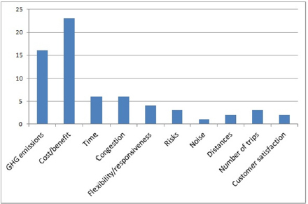
Figure 3.2. Opportunities for transport pooling
Logistics pooling is one of the strategies used to improve competitiveness and bring benefits to all stakeholders. Based on the results of the articles studied, we can see the rarity of articles dealing with purely vertical collaboration on one side, and on the other, we can see that the majority of articles refer either to horizontal collaboration or to integrated horizontal and vertical collaborations. Figure 3.2 shows the opportunities for transport pooling.
The pooling of transport has a positive effect on:
- – Economic performance: through cost reduction, financial gains by 82%, logistics time reduction by 21%, and improved flexibility and responsiveness of transporters by 14%.
- – Environmental performance: through the reduction of GHG emissions by 57%, road congestion and occupation by 21%, and noise.
- – Social and societal responsibility: through the reduction of risks by 11%, the number of trips by 11%, the improvement of customer satisfaction by 7%, and the reduction of distances traveled by 7%.
It should be noted that the majority of articles mainly focus on economic gain and/or GHG reduction, but with less intensity on the social and societal sides. However, among these opportunities, several have a strong interaction and can have effects on all three aspects of sustainability:
- – GHG emissions can be related to economic performance (CO2 tax, fuel costs, etc.). Similarly, reducing it is part of social responsibility (smog, health of residents, etc.).
- – Congestion increases GHG emissions, noise, time loss, fuel consumption, driver stress, customer dissatisfaction in the event of delays, accident risks, and so on.
- – Reducing distances and the number of trips leads to a reduction in fuel consumption, GHG emissions, and costs, saved time, better use of resources (less depreciation of trucks), better working conditions for drivers, and so on.
It can, therefore, be deduced that pooling and logistical collaboration make it possible to:
- – reduce logistics costs;
- – reduce GHG emissions;
- – reduce logistics times;
- – reduce congestion;
- – improve the flexibility and responsiveness of transporters;
- – reduce risks;
- – optimize the use of resources (number of trucks, distances traveled, loading, etc.).
At present, manufacturers are aware of the importance of optimizing their supply chain. This optimization is based on an economic approach, which is manifested through the integration of economic, environmental, and social concerns, which in turn are in line with the objectives of sustainable development. Thus, the environmental and societal degradation that goes hand in hand with economic development calls for serious action by all stakeholders, including regulators such as government, industry operators, and consumers.
In this context, the literature review shows that the majority of authors used scenarios as the initial source of knowledge for their analysis, with a rate of 57%. However, other sources are also used, such as hypotheses, questionnaires, and empirical data. In order to analyze the initial knowledge, the authors used a variety of tools and methods (both accurate or approximate). This majority opted for simulation in order to validate their basic proposal, with a rate of 35%. Figure 3.3 shows the methods based on mathematical models such as statistical analysis, linear programming, and heuristics/metaheuristics with a rate of 18% each. Similarly, Shapley optimization and values were also used with a rate of about 11% each.
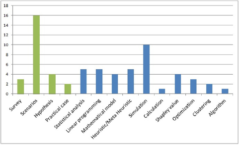
Figure 3.3. Analysis tools and methods used. For a color version of this figure, see www.iste.co.uk/besbes/transport.zip
In most of the articles on how to deal with problems, the most notable approach is to first propose scenarios and validate them, and then to use a single analytical method such as simulation (Chan and Zhang 2011; Junior et al. 2019; Thompson and Hassall 2012), linear programming (Muñoz-Villamizar et al. 2015; Pan 2010), metaheuristics (Abbassi et al. 2018), the Shapley value (Vanovermeire et al. 2013), optimization (Wang et al. 2019), and the algorithm (Perez-Bernabeu et al. 2015); or two methods, such as the mathematical model/simulation (Gonzalez-Feliu and Battaia 2017; Gonzalez-Feliu and Salanova 2012), metaheuristics/simulation (Gonzalez-Feliu 2011), linear programming/simulation (Danloup et al. 2015), and mathematical model/optimization (Silbermayr et al. 2017). On the other hand, Gonzalez-Feliu et al. (2013) used three methods to analyze the scenarios they proposed: namely, metaheuristics, clustering, and the Shapley value. In addition, some other authors adopted questionnaires and/or hypotheses and validated them with statistical analysis (Alvarez et al. 2018; Cao and Zhang 2010; Chen et al. 2013; Ghaderi et al. 2012).
3.5. Proposal of pooling scenarios for the urban distribution of goods
Pooling in the distribution phase consists of bringing together means of transport, warehouses, distribution centers, and, of course, information. Before focusing on pooling scenarios, we will emphasize on a scenario where companies do not use this technique: see Figure 3.4.

Figure 3.4. Scenario 0 without urban pooling. For a color version of this figure, see www.iste.co.uk/besbes/transport.zip
The scenarios are based on the following assumptions:
- – The trucks used have a maximum load of 3 and 9 tons.
- – The demand is equal to the supply. The three manufacturers each supply 1 ton of their product to each of the three customers.
- – The trajectories are recorded for the round trip (loaded truck)/(empty truck).
In scenario 0 (Figure 3.4), each manufacturer distributes 3 tons of its product with its own 3-ton truck. They make a trip to deliver a ton of product to each customer.
In scenario 1 (Figure 3.5), each manufacturer uses its own vehicle to transport the products to the transfer hub, where the three manufacturers exchange their products so that each truck is loaded with one ton of each type of product. A forklift truck ensures the transfer of products between the three trucks in seven operations, as shown in Figure 3.6. Each truck delivers its load to one of the three customers and returns to the owner company, either through the hub (S1) or through the shortest route (S1a).
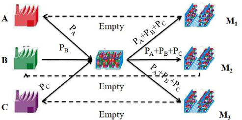
Figure 3.5. Scenario 1 of urban pooling. For a color version of this figure, see www.iste.co.uk/besbes/transport.zip
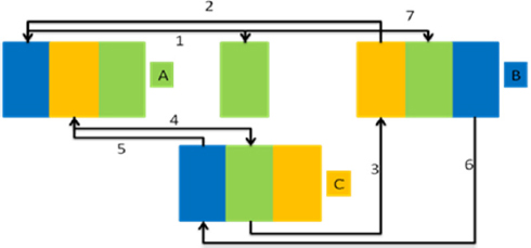
Figure 3.6. Exchange of products in the warehouse. For a color version of this figure, see www.iste.co.uk/besbes/transport.zip
In scenario 2 (Figure 3.7), as in scenario 1, each manufacturer uses its own 3-ton truck to transport its product to the warehouse. Subsequently, the distribution of different types of products is done in the form of a tour. The tour can either be done with a single rented 9-ton truck (S2a) or with three trucks, after having exchanged products with each other (S2).
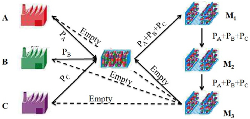
Figure 3.7. Scenario 2 of urban pooling. For a color version of this figure, see www.iste.co.uk/besbes/transport.zip
Scenario 3 (Figure 3.8) relates to the pooling of information and physical flows. Transport to the warehouse is done with a single vehicle, in the form of a tour. The warehouse then supplies each of the customers using a different vehicle. Therefore, in order to supply the hub with 3 tons of each product, either a 3-ton truck is used in three tours (S3) or a 9-ton truck is used in a single tour (S3a).

Figure 3.8. Scenario 3 of urban pooling. For a color version of this figure, see www.iste.co.uk/besbes/transport.zip
In scenario 4 (S4), as shown in Figure 3.9, company B is used as a consolidation center: all products are gathered in this center. A forklift performs the transfer (Figure 3.10), loading the three trucks with 1 ton of each product. Each truck loaded with the three types of product serves a different customer and returns empty to the owner company.

Figure 3.9. Scenario 4 of urban pooling. For a color version of this figure, see www.iste.co.uk/besbes/transport.zip
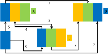
Figure 3.10. Transfer of products to B. For a color version of this figure, see www.iste.co.uk/besbes/transport.zip
As in scenario 4, Company B is used as a consolidation center for scenario 5: see Figure 3.11.

Figure 3.11. Scenario 5 of urban pooling. For a color version of this figure, see www.iste.co.uk/besbes/transport.zip
In this case, the first part is similar to scenario 4, but the distribution of the different products to customers’ stores is done in the form of tours, either using three 3-ton trucks, one from each company, (S5) or a 9-ton truck from company B (S5a). In the first case, the loading/unloading is similar to scenario 4, whereas in the second case, the forklift unloads the two trucks from A and C into the 9-ton truck and completes the load with 3 tons of product B.
Scenario 6 (Figure 3.12) involves making tours between manufacturers and customers. A 3-ton truck is supplied with one-third of its capacity each time it passes through a manufacturer. This truck continues its tour to the customers in order to deliver one-third of its load of A, B, and C products to each customer. In this case, either three tours are made with a single 3-ton truck or three 3-ton trucks (S6) are used. The tour can also be done with a 9-ton truck (S6a). Like in scenario 3, this scenario uses information pooling.
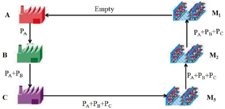
Figure 3.12. Scenario 6 of urban pooling. For a color version of this figure, see www.iste.co.uk/besbes/transport.zip
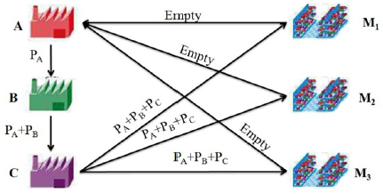
Figure 3.13. Scenario 7 of urban pooling. For a color version of this figure, see www.iste.co.uk/besbes/transport.zip
In scenario 7 (S7), as shown in Figure 3.13, the three 3-ton trucks leave from company A to C while passing through company B. At each company, they supply themselves with one-third of their loads with a type of product. Each truck then supplies a customer and returns to company A.
3.6. Comparison of scenarios
Now that these scenarios have been discussed, we can choose the best one based on the distance traveled by the vehicles. The shorter the distance, the lower the cost of transportation and GHG emissions. In addition, the lower the number of trucks used, the lower the congestion and the higher the truck operating rate will be.
3.6.1. Distances traveled
Figure 3.14 shows the distances between different organizations.
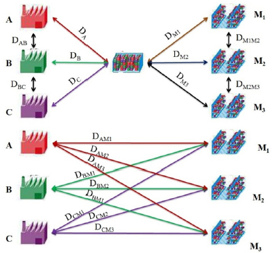
Figure 3.14. Distances between different organizations. For a color version of this figure, see www.iste.co.uk/besbes/transport.zip
For the rest of the study, we can consider the following assumptions:
- – The companies and the warehouse use trucks with a capacity of 3 or 9 tons.
- – Each manufacturer, A, B, and C, supplies 3 tons of its product (PA, PB, and PC).
- – Each customer, M1, M2, and M3, receives 1 ton of each product type.
- – Di (i = A, B, C) is the distance between company i and the hub.
- – DMj (j = 1, 2, 3) is the distance between the hub and customer Mj.
- – DAB is the distance between manufacturer A and manufacturer B.
- – DBC is the distance between manufacturer B and manufacturer C.
- – DM1M2 is the distance between client M1 and client M2.
- – DM2M3 is the distance between client M2 and client M3.
- – DiMj is the distance between company i and customer Mj.
To calculate the travel distances of the different scenarios, a Microsoft Excel spreadsheet is used, as shown in Figure 3.15. We simply enter the distances between organizations (Table 3.3) in order to get all the travel distances for the different scenarios, based on the shortest route, which can be determined by Google Maps. The results showed that each scenario could be the shortest route based on the distances between organizations.

Figure 3.15. Travel distances of the scenarios. For a color version of this figure, see www.iste.co.uk/besbes/transport.zip
Table 3.3. Distances between organizations
| DA | DB | DC | DM1 | DM2 | DM3 | DAB | DBC | DM1M2 | DM2M3 | DAMI | DAM3 | DBM1 | DBM3 | DCM1 | DCM3 | DBM2 | DCM2 | DAM2 |
| 10 | 12 | 8 | 15 | 10 | 14 | 7 | 4 | 8 | 6 | 18 | 20 | 15 | 14 | 21 | 19 | 12 | 16 | 20 |
It is worth mentioning that in Figure 3.15, scenario S2 has the shortest route (96 km) when using 3-ton trucks. In addition, it should be noted that with 9-ton trucks, all scenarios (S2a, S3a, S5a, and S6a) are slower than that with 3-ton, and hence, scenario S6a is the shortest route.
3.6.2. Greenhouse gas emissions
To calculate the CO2 equivalent (EqCO2) of exhaust emissions from trucks (CH4, Cox, etc.), the following formula is used:
where Fern is the mean EqCO2 emission factor for a diesel engine (kg/L) and Conso is the mean fuel consumption (L).
To calculate consumption (Conso), a recognized modeling that meets the standard BP X 30-323 (2015) is used, as shown by equation [3.2]1.
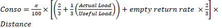
where (x) is the consumption of the full truck expressed in L/100 km, 2/3 of the consumption is related to the empty weight, and 1/3 of the consumption is related to the loaded weight.
The consumption (x) of a 3-ton truck is 15 L/100 km and that of the 9-ton truck is 25 L/100 km.
The Fern amounts to 2.662 EqCO2/L of fuel (diesel)2.
As for the calculation of the travel distances of the different scenarios, a Microsoft Excel spreadsheet is used to calculate the EqCO2 for each scenario, keeping the same inter-organizational distances, as shown in Figure 3.16. The results show that scenario S4 is the least expensive despite the fact that it is neither the shortest nor the least polluting scenario.

Figure 3.16. EqCO2 for the different scenarios
3.6.3. Distribution cost
The distribution cost (Ct Dist) is determined on the basis of the transport cost and the handling cost (loading and unloading), as shown by equation [3.3]:
The transport cost (Ct Tr) is calculated according to the distance of the journey traveled and the unit cost of the means of transport (3-ton or 9-ton truck, rented or not), as shown by equation [3.4].
where journey C3T is the course traveled by a 3-ton truck (km), journey C9T is the course traveled by a 9-ton truck (km), journey Dist C3T is the course traveled by a 3-ton truck from the distributor, Ctu C3T is the unit cost of transport by a 3-ton truck (DT/km), Ctu C9T is the unit cost of transport by a 9-ton truck (DT/km), and Ctu Dist C3T is the unit cost of transport by a 3-ton truck from the distributor (DT/km).
The cost of loading and unloading is a based on the amount that is loaded/unloaded and the relative time for loading and unloading a ton of product, in addition to the hourly cost of the handling equipment. The loading time (t Ch) is calculated by the following formula [3.5]:
where Charge C is the number of tons loaded/unloaded, Nb Ch is the number of times that Charge C has been repeated, and time Ch/T is the loading time for 1 ton of product.
The loading cost (Ct Ch) is the product of the loading time and the hourly cost of the handling equipment (equation [3.6]).
The equations are processed by an Excel sheet for the different scenarios, and the results are shown in Figure 3.17.
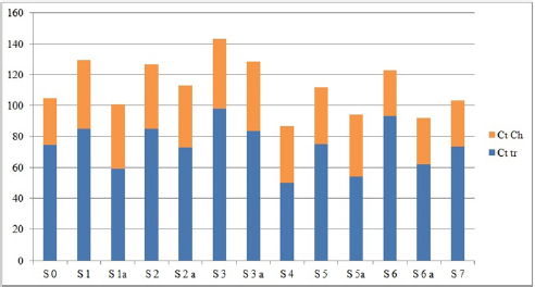
Figure 3.17. Distribution costs for the different scenarios. For a color version of this figure, see www.iste.co.uk/besbes/transport.zip
3.6.4. Delivery time
The delivery time (t Liv) is the sum of the transport times (ttr) and the loading time (t Ch), as shown by equation [3.7].
where (t Ch) is the total loading/unloading time, as shown by equation [3.5], and ∑ ttr is the sum of transport times (ttr) without counting the returns, as shown by equation [3.8].
where journey is the maximum distance of a 3-ton and/or 9-ton truck from the manufacturer to the customer without counting the return, and Vmoy is the mean speed (day or night) of a 3-ton and/or 9-ton truck.
On the Excel sheet, the equations are processed for the different scenarios. The results, which are presented in Figure 3.18, show that for the same inter-organizational distance setup as in the previous section, scenario S7 has the shortest delivery time with a duration of 4.28 h.
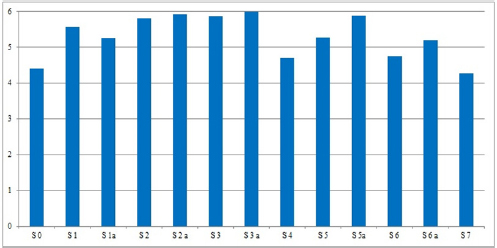
Figure 3.18. Delivery times for the different scenarios
3.6.5. Best scenario
With different Excel sheets, we have built a spreadsheet to calculate the values of different variables for all scenarios (EqCO2), distribution cost, and delivery time). However, the variables have different units, which makes it quite difficult to choose the optimal scenario. In order to overcome this problem, we have opted to calculate ratios relating to each criterion. The ratio (Rat) is calculated using the relationship between the value found and the maximum value of the studied variable (in other words, for (EqCO2, Rat Eq COe = EQ CO2i / Max (EQ CO21,. EQ CO2n) and i = 1 to n). To this extent, the optimal scenario will be the one that has the minimum sum of the ratios of different variables, given that all variables are looking to be minimized. The results of the Excel sheet (as shown in Figure 3.19), which make it possible to calculate the ratios of various criteria and help choose the optimal scenario, show that scenario S4 is the best choice.
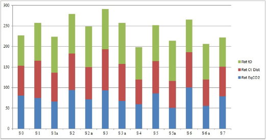
Figure 3.19. Comparison of the different scenarios. For a color version of this figure, see www.iste.co.uk/besbes/transport.zip
3.7. Proposal for a shared long-distance distribution model
The scenarios for pooling urban distribution, which have already been mentioned, have shown the role of pooling in reducing congestion and GHG emissions. The combination of urban and interurban distributions can generate more significant improvements. Therefore, the model we are going to propose is four cities. In each city, there are manufacturers and a consolidation warehouse that manages urban and/or interurban distribution to customers.
In scenario 1 (Figure 3.20), manufacturers in the same city transport their shipments to a warehouse that will then deliver individual orders for each customer in the city. In addition, the warehouse transports collective orders from customers in other cities through the relative warehouses. When returning, the trucks bring back collective orders from customers in the warehouse of departure from the first warehouse destination.
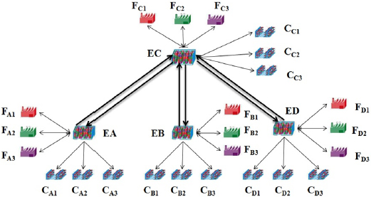
Figure 3.20. Scenario 1. For a color version of this figure, see www.iste.co.uk/besbes/transport.zip
For example, manufacturers in City A (FAi) transport their products to the EA warehouse, which distributes them to customers CAi and FAj, and to the EC warehouse which in turn distributes them to customers in the city (CCi and FCi) and to other corresponding EB and ED warehouses. When returning to the EC warehouse, the trucks transport the goods to the EA warehouse. Therefore, each customer/manufacturer in each city receives all products from all manufacturers located in their city or elsewhere.
In scenario 2 (Figure 3.21), FAi manufacturers transport their products to the EA warehouse for distribution to CAi customers and to the EB warehouse, which in turn distributes them to CBi customers and the EC warehouse. Upon return, trucks from the EA warehouse will be loaded with products from the EB warehouse network (FBi manufacturers and the EC warehouse can receive products from FCi and FDi manufacturers) to be delivered to customers in the EA warehouse. Therefore, customers in City A can receive products from all manufacturers (FAi, FBi, FCi, and FDi), and in addition to this, FAi manufacturers receive their supplies that have been manufactured in other cities.
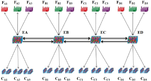
Figure 3.21. Scenario 2. For a color version of this figure, see www.iste.co.uk/besbes/transport.zip
The combination of the two scenarios allows us to implement our model presented in Figure 3.22.

Figure 3.22. Urban and interurban pooling models. For a color version of this figure, see www.iste.co.uk/besbes/transport.zip
This model can generate benefits for all stakeholders. The most significant advantage is that vehicles do not make empty returns, which leads to improved service efficiency, reduced GHG emissions, reduced road occupancy rates, better resource optimization (inventory, trucks, etc.), and reduced logistics costs.
In addition, this model clearly shows the role that pooling has in reducing GHG emissions – by reducing the number of vehicles used – and also in reducing congestion, given that pooling warehouses only allow small vehicles to be used in the city center.
3.8. Conclusion
The scenarios which we have suggested make it possible to identify some opportunities for transport pooling, such as the reduction of congestion and GHG emissions, while also considering the economic and social opportunities and gains. The comparison between the pooling scenarios and the scenario in which pooling is absent makes it possible to clearly show the improvements made by pooling transport in terms of distribution. The spreadsheet allows employees to choose the optimal scenario by considering different sustainability variables that lead to more efficient guidelines.
In conclusion, this is a multi-criteria decision support study using the following criteria: the cost of transportation (based on distance traveled), GHG emissions (based on distance traveled and truck characteristics), congestion (based on the number of trucks used), use of resources (based on the number of trucks used), and delivery time (based on distance, number of trucks used, and congestion). In addition, we plan discrete event simulations in order to consider the random concept of transport times in any distribution function.
3.9. References
Abbad, H. (2014). La gestion mutualisée des approvisionnements : mythe ou réalités? Logistique & Management, 22(2), 41–50.
Abbad, H., Durand, B., and Senkel M.-P. (2016). La mutualisation physique et informationnelle en logistique. In Organisation, Information et Performance, Meyssonnier, F. and Rowe, F. (eds). Editions PUR, Rennes.
Abbassi, A., Kharraja, S., Alaoui, A.E., and Parra, D. (2018). Comparative study of mutualisation scenarios for distribution of non-medical products. 3rd SCA International Conference on Smart City Applications, Tetouan, Morocco.
AFNOR. (2015). Principes généraux pour l’affichage environnemental des produits de grande consommation – Partie 0 : principes généraux et cadre méthodologique. Report, no. BP BP X 30-323, Agence De l’Environnement et de la Maitrise de l’Energie (ADEME), Angers, France.
Alvarez, P., Serrano-Hernandez, A., Faulin, J., and Juan, A.A. (2018). Using modelling techniques to analyze urban freight distribution. A case study in Pamplona (Spain). Transportation Research Procedia, 33, 67–74.
Bahinipati, B.K., Kanda, A., and Deshmukh, S.G. (2009). Horizontal collaboration in semiconductor manufacturing industry supply chain: an evaluation of collaboration intensity index. Computers & Industrial Engineering, 57(3), 880–895.
Ballot, E. and Fontane, F. (2008). Reducing transportation CO2 emissions through pooling of supply networks: perspectives from a case study in French retail chains. Production Planning & Control: the Management of Operations, 21(6), 640–650.
Bustinza, O.F., Gomes, E., Vendrell-Herrero, F., and Baines, T. (2019). Product–service innovation and performance: the role of collaborative partnerships and R&D intensity. R&D Management, 49(1), 33–45.
Camarinha-Matos, L.M. (2014). Collaborative networks: a mechanism for enterprise agility and resilience. In Enterprise Interoperability VI: Interoperability for Agility, Resilience and Plasticity of Collaborations, Proceedings of the I-ESA Conferences, Mertins, K., Benaben, F., Poler, R., and Bourrières, J.-P. (eds). Springer International Publishing, Cham.
Cao, M. and Zhang, Q. (2010). Supply chain collaboration: impact on collaborative advantage and firm performance. Journal of Operations Management, 29(3), 163–180.
Chan, F.T.S. and Zhang, T. (2011). The impact of Collaborative Transportation Management on supply chain performance: a simulation approach. Expert Systems With Applications, 38(3), 2319–2329.
Chanut, O. and Paché, G. (2013). La culture de mutualisation du PSL peut-elle favoriser l’émergence d’une logistique urbaine durable? RIMHE: Revue Interdisciplinaire Management, Homme Entreprise, 3, 94–110.
Chanut, O., Capo, C., and Bonet, D. (2010). La mutualisation des moyens logistiques ne concerne-t-elle que les grandes entreprises? Le point des pratiques dans les systèmes verticaux contractuels. 8èmes RIRL Rencontres Internationales de la Recherche en Logistique, Bordeaux, France, September–October.
Chay, Y., Chanut, O., Michon, V., and Roques, T. (2013). La mutualisation logistique pour des Supply Chains durables. In La logistique: une approche innovante des organisations, Fabbe-Costes, N. and Pache, G. (eds). Presse Universitaire de Provence, Aix-en-Provence.
Chen, J., Sohal, A.S., and Prajogo, D.-I. (2013). Supply chain operational risk mitigation: a collaborative approach. International Journal of Production Research, 51(7), 2186–2199.
Cleophas, C., Cottrill, C., Ehmke, J.F., and Tierney, K. (2019). Collaborative urban transportation: recent advances in theory and practice. European Journal of Operational Research, 273(3), 801–816.
Danloup, N., Mirzabeiki, V., Allaoui, H., Goncalves, G., Julien, D., and Mena, C. (2015). Reducing transportation greenhouse gas emissions with collaborative distribution: a case study. Management Research Review, 38(10), 1049–1067.
Destouches, G. and Gaide, F. (2011). Pratiques de logistique collaborative: quelles opportunités pour les PME/ETI? Report, Pôle interministériel de prospective et d’anticipation des mutations économiques (PIPAME).
Fernandez, E., Fontana, D., and Speranza, M.G. (2016). The Collaboration Uncapacitated Arc Routing Problem. Computers and Operation Research, 67, 120–167.
Ghaderi, H., Darestani, S.A., Leman, Z., and Ismail, M. (2012). Horizontal collaboration in logistics: a feasible task for group purchasing. International Journal of Procurement Management, 5(1), 43–54.
Ghaderi, H., Dullaert, W., and Amstel, W.P.V. (2016). Reducing lead-times and lead-time variance in cooperative distribution networks. International Journal of Shipping and Transport Logistics, 8(1), 51–65.
Gharehgozli, A.H., De Koster, R., and Jansen, R. (2017). Collaborative solutions for inter terminal transport. International Journal of Production Research, 55(21), 6527-6546.
Gonzalez-Feliu, J. (2011). Costs and benefits of logistics pooling for urban freight distribution: scenario simulation and assessment for strategic decision support. Seminario CREI, Rome, Italy.
Gonzalez-Feliu, J. and Battaia, G. (2017). La mutualisation des livraisons urbaines : quels impacts sur les coûts et la congestion? Logistique & Management, 25(2), 107–118.
Gonzalez-Feliu, J. and Salanova, J. (2012). Defining and evaluating collaborative urban freight distribution systems. Procedia – Social and Behavioral Science, 39, 172–183.
Gonzalez-Feliu, J., Morana, J., Grau, J.-M.S., and Ma, T.-Y. (2013). Design and scenario assessment for collaborative logistics and freight transport systems. International Journal of Transport Economics/Rivista internazionale di economia dei trasporti, 4(2), 207–240.
Guajardo, M. and Rönnqvist, M. (2016). A review on cost allocation methods in collaborative transportation. International Transactions in Operational Research, 23(3), 371–392.
Hadj Taieb, N., Mellouli, R., and Affes, H. (2014). Impact of means and resources pooling on supply-chain management: case of large distribution. 3rd IEEE ICALT’14, International Conference on Advanced Logistics and Transport, Hammamet, Tunisia.
Hensher, D.A. (2018). Tackling road congestion – what might it look like in the future under a collaborative and connected mobility model. Transport Policy, 66, A1–A8.
Junior, D.P.A., Novaes, A.G.N., and Luna, M.M.M. (2019). An agent-based approach to evaluate collaborative strategies in milk-run OEM operations. Computers & Industrial Engineering, 129, 545–555.
Liakos, P. and Delis, A. (2015). An interactive freight-pooling service for efficient last-mile delivery. 16th IEEE International Conference on Mobile Data Management, Pittsburgh, USA.
Liu, D., Deng, Z., Sun, Q., Wang, Y., and Wang, Y. (2019). Design and freight corridor-fleet size choice in collaborative intermodal transportation network considering economies of scale. Sustainability, 11(4), 990–1008.
Lundqvist, B. (2018). Data collaboration, pooling and hoarding under competition law. Faculty of Law, Stockholm University Research Paper.
McKinnon, A. and Edwards, J. (2010). Opportunities for improving vehicle utilization. In Green Logistics: Improving the Environmental Sustainability of Logistics, McKinnon, A., Cullinane, S., Browne, M., and Whiteing, A. (eds). Kogan Page Publisher, London.
Moharana, H.S., Murty, J.S., Senapati, S.K., and Khuntia, K. (2012). Coordination, collaboration and integration for supply chain management. International Journal of Interscience Management Review, 2(2), 46–50.
Moutaoukil, A., Derrouiche, R., and Neubert, G. (2012). Pooling supply chain: literature review of collaborative strategies. 13th Working Conference on Virtual Enterprises, Bournemouth, UK.
Moutaoukil, A., Derrouiche, R., and Neubert, G. (2013). Modélisation d’une stratégie de mutualisation logistique en intégrant les objectifs de Développement Durable pour des PME agroalimentaires. 13e CIGI’13 Congrès International de Génie Industriel, La Rochelle, France.
Moutaoukil, A., Neubert, G., and Derrouiche, R. (2015). Urban freight distribution: the impact of delivery time on sustainability. IFAC-PapersOnLine, 48(3), 2368–2373.
Muñoz-Villamizar, A., Montoya-Torres, J.R., and Vega-Mejía, C.A. (2015). Non-collaborative versus collaborative last-mile delivery in urban systems with stochastic demands. Procedia CIRP, 30, 263–268.
Murça, M.C.R. (2018). Collaborative air traffic flow management: incorporating airline preferences in rerouting decisions. Journal of Air Transport Management, 71, 97–107.
Niu, F. and Li, J. (2019). An activity-based integrated land-use transport model for urban spatial distribution simulation. Environment and Planning B: Urban Analytics and City Science, 46(1), 165–178.
Ntziachristos, L., Papadimitriou, G., Ligterink, N., and Hausberger, S. (2016). Implications of diesel emissions control failures to emission factors and road transport NOx evolution. Atmospheric Environment, 141, 542–551.
Okdinawati, L., Simatupang, T.M., and Sunitiyoso, Y. (2015). Modelling collaborative transportation management: current state and opportunities for future research. Journal of Operations and Supply Chain Management, 8(2), 96–119.
Pan, S. (2010). Contribution à la définition et à l’évaluation de la mutualisation de chaînes logistiques pour réduire les émissions de CO2 du transport : application au cas de la grande distribution. PhD thesis, École Nationale Supérieure des Mines, Paris.
Pan, S., Ballot, E., and Fontane, F. (2013). The reduction of greenhouse gas emissions from freight transport by pooling supply chains. International Journal Production Economics, 143(1), 86–94.
Perboli, G., Rosano, M., and Gobbato, L. (2016). Decision support system for collaborative freight transportation management: a tool for mixing traditional and green logistics. 6th ILS International Conference on Information Systems, Logistics and Supply Chain, Bordeaux, France.
Perez-Bernabeu, E., Juan, A.A., Faulin, J., and Barrios, B.B. (2015). Horizontal cooperation in road transportation: a case illustrating savings in distances and greenhouse gas emissions. International Transactions in Operational Research, 22(3), 585–606.
Qiu, X. and Huang, G.Q. (2011). On storage capacity pooling through the supply hub in industrial park (SHIP): the impact of demand uncertainty. IEEM’2011 IEEE International Conference on Industrial Engineering and Engineering Management, Singapore.
Rajaa, M. and Ibnoulkatib, G. (2019). La logistique urbaine: identification des concepts clés (revue de littérature). European Scientific Journal, 15(2), 57–71.
Rakotonarivo, D., Gonzalez-Feliu, J., Aoufi, A., and Morana, J. (2009). La mutualisation. Report, LUMD: Logistique Urbaine Mutualisée Durable, Université Lyon 2. Available: https://halshs.archives-ouvertes.fr/halshs-01056188.
Sanchez, M., Pradenas, L., Deschamps, J.-C., and Parada, V. (2016). Reducing the carbon footprint in a vehicle routing problem by pooling resources from different companies. NETNOMICS: Economic Research and Electronic Networking, 17(1), 29–45.
Senkel, M.-P., Durand, B., and Hoa Vo, T.L. (2013). La mutualisation logistique : entre théories et pratiques. Logistique & Management, 21(1), 19–30.
Silbermayr, L., Jammernegg, W., and Kischka, P. (2017). Inventory pooling with environmental constraints using copulas. European Journal of Operational Research, 263(2), 479–492.
Tellez, O., Vercraene, S., Lehuede, F., Peton, O., and Monteiro, T. (2016). Optimisation du transport mutualisé d’enfants en situation de handicap avec véhicules reconfigurables. ROADEF’2016 17e congrès de la société Française de Recherche Opérationnelle et d’Aide à la Décision, Compiègne, France, February.
Thompson, R.G. and Hassall, K.P. (2012). A collaborative urban distribution network. Procedia – Social and Behavioral Sciences, 39, 230–240.
Tornberg, P. and Odhage, J. (2018). Making transport planning more collaborative? The case of Strategic Choice of Measures in Swedish transport planning. Transportation Research Part A: Policy and Practice, 118, 416–429.
Vanovermeire, C., Sörensen, K., Van Breedam, A., Vannieuwenhuyse, B., and Verstrepen, S. (2013). Horizontal logistics collaboration: decreasing costs through flexibility and an adequate cost allocation strategy. International Journal of Logistics: Research and Applications, 17(4), 339–355.
Wang, X. and Kopfer, H. (2014). Collaborative transportation planning of less-than-truckload freight. OR Spectrum, 36(2), 357–380.
Wang, Y., Ma, X., Li, Z., Liu, Y., Xu, M., and Wang, Y. (2017). Profit distribution in collaborative multiple centers vehicle routing problem. Journal of Cleaner Production, 144, 203-219.
Wang, X.-X., Liu, X.-Y., and Li, Z.-Q. (2018). A social collaborative urban distribution integration platform. Journal of Interdisciplinary Mathematics, 21(5), 1109–1113.
Wang, J., Lim, M.K., Tseng, M.-L., and Yang, Y. (2019). Promoting low carbon agenda in the urban logistics network distribution system. Journal of Cleaner Production, 211, 146-160.
Zissis, D., Aktas, E., and Bourlakis, M. (2018). Collaboration in urban distribution of online grocery orders. The International Journal of Logistics Management, 29(4), 1196–1214.
Zouari, A. and Cherif, M. (2018). La mutualisation des transports : cas de la distribution urbaine – Partie 1 revue de litérature. CESCA’2018, 1er Colloque International sur l’E-Supply Chain, Agadir, Morocco.
Chapter written by Alaeddine ZOUARI.