
3.6 Source localization in complex listening situations
In addition to the spatial hearing knowledge presented so far, for spatial audio processing and coding it is useful to understand how the auditory system determines the locations of sources in complex listening scenarios. The relation between interaural time difference (ITD) and interaural level difference (ILD) and source direction in free-field is obvious and a conclusion that the auditory system discriminates the source direction as a function of ITD and ILD is in this case rather plausible. However, some phenomena have also been described for which it is not obvious how the auditory system processes ear entrance signal properties for localization of sound sources. For example, when a number of sources are concurrently active, ITD and ILD are likely to be time varying and in many cases their values do not correspond directly to source directions. In an enclosed space, when sound from sources not only reaches the ears of a listener directly, but also indirectly from different directions, the matter of localization of the sources becomes even more complicated. Playback of ‘real-world’ stereo and multi-channel audio signals usually mimics listening to multiple concurrently active sources in rooms. For the task of spatial audio processing or designing a coding scheme for spatial audio it is helpful to understand which signal properties are important to the auditory system for source localization, source width, and envelopment perception. These properties need to be maintained when coding stereo and multi-channel audio signals in order that the auditory spatial image of the coded audio signal corresponds to the auditory spatial image of the original signal.
While single-source localization in the presence of reflections can be at least partially explained by the precedence effect, the attempt of the model, described in the following, is to explain source localization for the general case of multiple concurrently active sources and reflections. The model is denoted cue selection model and is described in greater detail in [87].
3.6.1 Cue selection model
In most listening situations, the perceived directions of auditory objects coincide with the directions of the corresponding physical sound sources. In everyday complex listening scenarios, sound from multiple sources, as well as reflections from the surfaces of the physical surroundings, arrive concurrently from different directions at the ears of a listener. The auditory system not only needs to be able to independently localize the concurrently active sources, but it also needs to be able to suppress the effect of the reflections. The cue selection model, described in the following, qualitatively explains both of these features.
The basic approach of the cue selection model is very straightforward: only ITD and ILD cues occurring at time instants when they represent the direction of one of the sources are selected, while other cues are ignored. The interaural coherence (IC) is used as an indicator for these time instants. More specifically, in many cases by selecting ITD and ILD cues coinciding with IC cues larger than a certain threshold, one obtains a subset of ITD and ILD cues similar to the corresponding cues of each source presented separately in free-field. The cue selection is implemented in the framework of a model that considers a physically and physiologically motivated peripheral stage, whereas the remaining parts are analytically motivated. Fairly standard binaural analysis is used to calculate the instantaneous ITD, ILD, and IC cues.
Model overview
The auditory system features a number of physical, physiological, and psychological processing stages for accomplishing the task of source direction discrimination and ultimately the formation of the auditory spatial image. The structure of a generic model for spatial hearing is illustrated in Figure 3.20. There is little doubt about the first stages of the auditory system, i.e. the physical and physiological functioning of the outer, middle, and inner ear are known and understood to a high degree. However, already the stage of the binaural processor is less well known. Different models have used different approaches to explain various aspects of binaural perception. The majority of proposed localization models are based on analysis of ITD cues using a coincidence structure [152], or a cross-correlation implementation that can be seen as a special case of the coincidence structure. Evidence for cross-correlation-like neural processing has also been found in physiological studies [280]. However, such excitation–excitation (EE) type cells are but one kind of neural units potentially useful for obtaining binaural information (see e.g. the introduction and references of [46] and Section 3.3). With current knowledge, the interaction between the binaural processor and higher level cognitive processes can be addressed only through indirect psychophysical evidence.
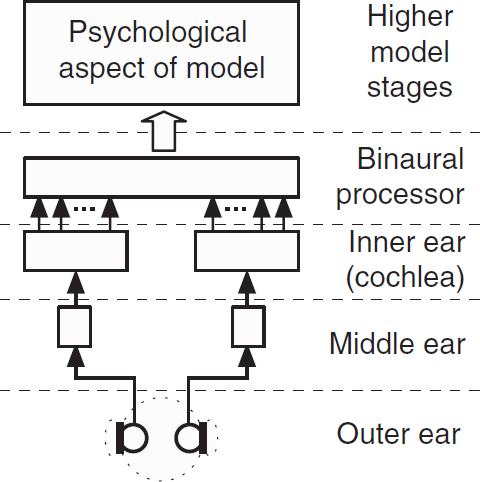
Figure 3.20 A model of spatial hearing covering the physical, physiological, and psychological aspects of the auditory system.
Auditory periphery
Transduction of sound from a source to the ears of a listener is modeled by filtering the source signals either with head-related transfer functions (HRTFs) or with measured binaural room impulse responses (BRIRs). HRTF filtering simulates the direction dependent influence of the head and outer ears on the ear input signals. BRIRs additionally include the effect of room reflections in an enclosed space. In multi-source scenarios, each source signal is first filtered with a pair of HRTFs or BRIRs corresponding to the simulated location of the source, and the resulting ear input signals are summed before the next processing stage.
The effect of the middle ear is typically described as a bandpass filter. The frequency analysis of the basilar membrane is simulated by passing the left and right ear signals through a gammatone filterbank [207]. An example of magnitude responses for a set of gammatone filters with center frequencies between about 500 and 2000 Hz are illustrated in Figure 3.21. Each resulting critical band signal is processed using a model of neural transduction, e.g. as described in Bernstein et al. [23]. The resulting nerve firing densities at the corresponding left and right ear critical bands are denoted x1 and x2.
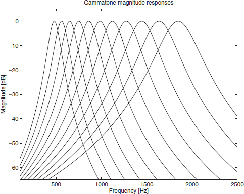
Figure 3.21 Magnitude responses for a set of gammatone filters with center frequencies of 10–20 ERB.
Internal noise is introduced into the model in order to describe the limited accuracy of the auditory system. For this purpose independent Gaussian noise, filtered with the same gammatone filters as the considered critical band signals, is added to each critical band signal before applying the model of neural transduction.
Binaural processor
The cue selection model in principle does not make a specific physiological assumption about the binaural processor. The only assumption is that its output signals (e.g. binaural activity patterns) yield information which can be used by the upper stages of the auditory system for discriminating ITD, ILD, and IC. Given this assumption, the cue selection model computes the ITD, ILD, and IC directly. Note that in this discussion ITD, ILD, and IC are defined with respect to critical band signals after applying the neural transduction. ITD, ILD and IC estimation is part of many existing models for sound source localization and binaural unmasking. Hence the proposed approach can in principle be integrated in many existing models.
The binaural cues are estimated with a running process as a function of time in each critical band. The ITD and IC are estimated from the normalized cross-correlation function Φ (n, m), where n is the time index and m is the lag index of the normalized cross-correlation function.
Choosing the time constant T for the running process to compute the binaural cues is a difficult task. Studies of binaural detection actually suggest that the auditory system integrates binaural data using a double-sided window with time constants of both sides in the order of 20–60 ms (e.g. [125, 167]). However, a double-sided window with this large time constant will not be able to explain the precedence effect, where the localization of a lead sound should not be influenced by a lagging sound after only a few milliseconds. The difference in the observed behavior for these different cases could be explained by assuming that the auditory system comprises multiple temporal analysis stages that have different time constants, or a system that can adapt its temporal resolution to the task that it has to perform. Here a single-sided exponential time window with a time constant of 10 ms is used, in accordance with the time constant of the temporal inhibition of the model of Lindemann [182].
Φ(n, m) is evaluated over time lags in the range of [−1,1] ms. The ITD (in samples) is estimated as the lag of the maximum of the normalized cross-correlation function,
![]()
The IC is defined as the maximum value of the instantaneous normalized crosscorrelation function,
![]()
This estimate describes the coherence of the left and right ear input signals. In principle, it has a range of [0,1], where 1 occurs for perfectly coherent left and right critical band signals. The neural transduction introduces a DC offset and thus the values of IC(n) are typically higher than 0 even for independent (nonzero) critical band signals.
The ILD is computed as the level difference between the left and right critical band signals in dB. Note that, due to the effect of neural transduction, the resulting ILD estimates will be smaller than the level differences between the ear input signals.
Higher model stages
A vast amount of information is available to the upper stages of the auditory system through the signals from the auditory periphery. The focus of the cue selection model lies only in the analysis of the three inter-channel properties between left and right critical band signals that were defined in the previous section: ITD, ILD, and IC. It is assumed that at each time instant n the information about the values of these three signal properties, is available for further processing in the upper stages of the auditory system.
Consider the simple case of a single source in free-field. Whenever there is sufficient signal power, the source direction determines the nearly constant ITD and ILD which appear between each left and right critical band signal. The (average) ITDs and ILDs occurring in this scenario are denoted free-field cues in the following. The free-field cues of a source with an azimuthal angle ϕ are denoted ITDϕ and ILDϕ. It is assumed that this kind of a one-source free-field scenario is the reference for the auditory system. That is, in order for the auditory system to perceive auditory objects at the directions of the sources, it must obtain ITD and/or ILD cues similar to the free-field cues corresponding to each source that is being discriminated. The most straightforward way to achieve this is to select the ITD and ILD cues at time instants when they are similar to the free-field cues. In the following it is shown how this can be done with the help of IC.
When several independent sources are concurrently active in free-field, the resulting cue triplets {ILD(n),ITD(n),IC(n)} can be classified into two groups. (1) Cues arising at time instants when only one of the sources has power in that critical band. These cues are similar to the free-field cues (direction is represented in {ILD(n),ITD(n)}, and IC(n) ≈ 1). (2) Cues arising when multiple sources have non-negligible power in a critical band. In such a case, the pair {ILD(n),ITD(n)} does not represent the direction of any single source, unless the superposition of the source signals at the ears of the listener incidentally produces similar cues. Furthermore, when the two sources are assumed to be independent, the cues are fluctuating and IC(n) < 1. These considerations motivate the following method for selecting ITD and ILD cues. Given the set of all cue pairs, {ILD(n),ITD(n)}, only the subset of pairs is considered which occurs simultaneously with an IC larger than a certain threshold, IC(n) > IC0. This subset is denoted
![]()
The same cue selection method is applicable for deriving the direction of a source while suppressing the directions of one or more reflections. When the ‘first wavefront’ arrives at the ears of a listener, the evoked ITD and ILD cues are similar to the free-field cues of the source, and IC(n) ≈ 1. As soon as the first reflection from a different direction arrives, the superposition of the source signal and the reflection results in cues that do not resemble the free-field cues of either the source or the reflection. At the same time IC reduces to IC <1, since the direct sound and the reflection superimpose as two signal pairs with different ITD and ILD. Thus, IC can be used as an indicator for whether ITD and ILD cues are similar to free-field cues of sources or not (while ignoring cues related to reflections).
For a given IC0 there are several factors determining how frequently IC(n) > IC0. In addition to the number, strengths, and directions of the sound sources and room reflections, IC(n) depends on the specific source signals and on the critical band being analyzed. In many cases, the larger IC0 the more similar the selected cues are to the free-field cues. However, there is a strong motivation to choose IC0 as small as possible while still getting accurate enough ITD and/or ILD cues, because this will lead to the cues being selected more often, and consequently to a larger proportion of the ear input signals contributing to the localization.
It is assumed that the auditory system adapts IC0 for each specific listening situation, i.e., for each scenario with a constant number of active sources at specific locations in a constant acoustical environment. Since the listening situations do not usually change very quickly, it is assumed that IC0 is adapted relatively slowly in time. In [87] it is also argued that such an adaptive process may be related to the buildup of the precedence effect. The simulations reported in the following consider only one specific listening situation at a time. Therefore, for each simulation a single constant IC0 is used.
It is assumed that for each specific listening situation the auditory system adapts IC0 until ITD and ILD cues representing source directions are obtained by the cue selection.
3.6.2 Simulation examples
As mentioned earlier, the cue selection model assumes that, in order to perceive an auditory object at a certain direction, the auditory system needs to obtain cues similar to the free-field cues corresponding to a source at that direction. In the following, the cue selection model is applied to several stimuli that have been used in previously published psychophysical studies. Both, the selected cues as well as all cues prior to the selection, are illustrated and the implied directions are discussed in relation to the literature. Many more simulations are presented in [87].
Usually, the larger the cue selection threshold c0, the smaller is the difference between the selected cues and the free-field cues. The choice of c0 is a compromise between the similarity of the selected cues to the free-field cues and the proportion of the ear input signals contributing to the resulting localization.
Here, application of the cue selection is only considered independently at single critical bands. Except for different values of c0, the typical behavior appears to be fairly similar at critical bands with different center frequencies. The listening situations are simulated using HRTFs. All simulated sound sources are located in the frontal horizontal plane and the stimuli are aligned to 60 dB SPL averaged over the whole stimulus length.
Independent sources in free-field
A speech source can still be rather accurately localized in the presence of one or more competing other speech sources, Hawley et al. [116] and Drullman and Bronkhorst [70]. Thus, to be correct, the cue selection has to yield ITD and ILD cues similar to the free-field cues of each of the speech sources in order to correctly predict the directions of the perceived auditory objects. A simulation was carried out with two concurrent speech sources. The signal of each source consisted of a different phonetically balanced sentence from the Harvard IEEE list [132] recorded by the same male speaker. The two speech sources were simulated at azimuthal angles of ±40°. Figure 3.22 shows the IC, ILD, and ITD as a function of time for the critical bands with center frequencies of 500 Hz and 2 kHz. The free-field cues which would occur with a separate simulation of the sources at the same angles are indicated with the dashed lines. The selected ITD and ILD cues (3.9) are marked with bold solid lines. Thresholds of c0 = 0.95 and c0 = 0.99 were used for the 500 Hz and 2 kHz critical bands, respectively, resulting in 65 and 54% selected signal power. The selected cues are always close to the free-field cues, implying perception of two auditory objects located at the directions of the sources, as reported in the literature. As expected, due to the neural transduction IC has a smaller range at the 2 kHz critical band than at the 500 critical band. Consequently, a larger c0 is required.
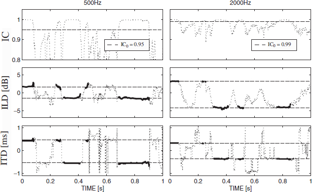
Figure 3.22 IC, ILD, and ITD as a function of time for two independent speech sources at ±40° azimuth. Left column 500 Hz; right column 2 kHz critical band. The cue selection thresholds (top row) and the free-field cues of the sources (middle and bottom rows) are indicated with dashed lines. Selected cues are marked with bold solid lines.
Precedence effect
In the following, the cue selection is illustrated within the context of the precedence effect. In a classical precedence effect experiment, a lead/lag pair of clicks is presented to the listener [26, 183]. The leading click is first emitted from one direction, followed by another identical click from another direction after an interclick interval (ICI) of a few milliseconds. For ICIs within a range of about 1 to 10 ms a listener perceives sound only from the direction of the leading click.
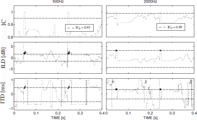
Figure 3.23 IC, ILD, and ITD as a function of time for a lead/lag click-train with a rate of 5 Hz and an ICI of 5 ms. Left column 500 Hz; right column 2 kHz critical band. The cue selection thresholds (top row) and the free-field cues of the sources (middle and bottom rows) are indicated with dashed lines. Selected cues are marked with bold solid lines.
Figure 3.23 shows IC, ILD, and ITD as a function of time for a click train with a rate of 5 Hz analyzed at the critical bands centered at 500 Hz and 2 kHz. The lead source is simulated at 40° and the lag at −40° azimuth with an ICI of 5 ms. As expected based on earlier discussion, IC is close to one whenever only the lead sound is within the analysis time window. As soon as the lag reaches the ears of the listener, the superposition of the two clicks reduces the IC. The cues obtained by the selection with c0 = 0.95 for the 500 Hz and c0 = 0.985 for the 2 kHz critical band are shown in the figure, and the free-field cues of both sources are indicated with dashed lines. The selected cues are close to the free-field cues of the leading source and the cues related to the lag are ignored (not selected), as is expected to happen based on psychophysical studies [183]. The fluctuation in the cues before each new click pair is due to the internal noise of the model.