9.3 Side information

The previously derived expressions for the inter-channel cues occurring when mixing the (original) source signals indicate which properties determine the inter-channel cues of the mixer output signal. The ICLD (Equation 9.6) depends on the mixing parameters (a_i, b_i) and on the short-time subband power of the sources, E{²(n)} (Equation 9.5). The normalized subband cross-correlation function Φ(n, d) (Equation 9.11), that is needed for ICTD (Equation 9.9) and ICC (Equation 9.8) computation, depends on E{²₁(n)} and additionally on the normalized sub-band autocorrelation function, Φ_i(n, e) (Equation 9.12), for each source signal. If no time adjustments are applied (i.e. c_i = d_i = 0), only subband powers are required, without autocorrelation functions. Finally, the level of the mixer output channels depends on the mixing parameters (a_i, b_i) and sub-band power of the sources E{²(n)(n)}.

Hence, given the rendering parameters (a_i, b_i, c_i, d_i), the spatial parameters of the rendered scene can be obtained based on the source subband powers E{²_i(n)} which hence have to be transmitted along with the down-mix signal s(n). In order to reduce the amount of side information, the relative dynamic range of the source signal parameters is limited. At each time, for each sub-band, the power of the strongest source is selected. It was found to suffice to lower bound the corresponding subband power of all the other sources at a value 24 dB lower than the strongest subband power. Thus, the dynamic range of the quantizer can be limited to 24 dB.

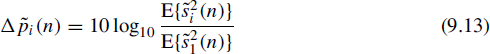
The power of the sources with indices 2 ≤ i ≤ M relative to the power of the first source is transmitted as side information,

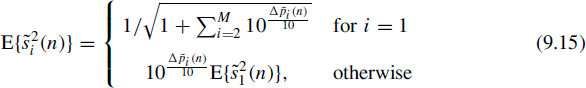
Note that dynamic range limiting as described previously is carried out prior to Equation (9.13), avoiding numerical problems when E{²₁(n)} vanishes. A total of 20 sub bands was used in combination with a parameter update rate for each subband Δ_i(n) (2 ≤ i ≤ M) of about 12 ms. The relative power values are quantized and Huffman coded, resulting in a bitrate of approximately 3(M − 1) kb/s [84].

9.3.1 Reconstructing the sources

Figure 9.5 illustrates the process that is used to re-create the source signals, given the sum signal (Equation 9.1). This process is part of the ‘Synthesis’ block in Figure 9.2. The individual source signals are recovered by scaling each sub-band of the sum signal with g_i(n) and by applying a decorrelation filter with impulse response h_i(n),

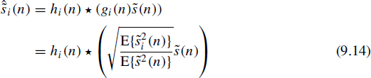
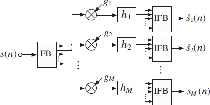
Figure 9.5 The process for generation of ŝ_i(n). The sum signal is converted to the sub-band domain. The sub-bands are scaled such that the sub-band power is approximately the same as the sub-band power of the original source signals. Filtering is applied to the scaled sub-bands for decorrelation. The shown processing is carried out independently for each sub-band. FB is a filterbank with sub-bands with bandwidths motivated by perception. IFB is the corresponding inverse filterbank.

where * is the linear convolution operator and E{²_i (n)} is computed with the side information by

As decorrelation filters h_i(n), complementary comb filters [179], allpass filters [79, 232], delays [34], or filters with random impulse responses [82, 83] may be used. The goal for the decorrelation process is to reduce correlation between the signals while not modifying how the individual waveforms are perceived. Different decorrelation techniques cause different artifacts. Complementary comb filters cause coloration. All the described techniques are spreading the energy of transients in time causing artifacts such as ‘preechoes’. Given their potential for artifacts, decorrelation techniques should be applied as little as possible.

When applying no decorrelation processing (h_i(n) = δ(n) in Equation (9.14)) good audio quality can also be achieved. It is a compromise between artifacts introduced by the decorrelation processing and artifacts due to the fact that the source signals ŝ_i(n) are correlated. In fact, it is only beneficial to reconstruct ICC at the mixer output rather than the mixer input signals (i.e. the recovered source signals) by integrating the source estimation and mixing processes in the parametric domain, as outlined in the next section.