8.1 Introduction

When running linear regressions we can explain the influence on a dependent metric variable in a fashion like “People who are union members earn on average 1.5 $ more per hour than other people.” Pay attention to the metric of our prediction, which is measured in dollars, years, points or any other metric unit. When we deal with binary variables this is no longer possible, and we have to start thinking in probabilities. In a logistic regression, an independent variable can only influence the probability of going from one state (0) to the other (1).

In our example we want to research the effect of age on the chance of having a heart attack. The coding of the dependent variable is binary: people either had a heart attack or not, therefore, we use a logistic model. The independent variable is metric. Note that the arrow of causation can only point in one direction, as age can cause heart attacks, but heart attacks cannot cause (or influence) age. We will also introduce control variables, to account for spurious correlations.

To see the method in action, we will load another dataset which is taken from the second National Health and Nutrition Examination Survey (NHANES II)56 which surveyed people in the USA about their health and diets between 1976 and 1980. We will use a sample of the data, which is not representative of the general population of the USA. Furthermore, we will ignore the sampling design, which introduces bias. Consequently, our results will not be valid in general or meet scientific standards, yet will be adequate for the purpose of demonstrating the technique. We open the dataset by typing

webuse nhanes2, clear

First we inspect our dependent variable (heartatk) and our central independent variable (age), to get an impression of the general distribution of the data

tabulate heartatk

summarize age, detail

We see that about 4.6% of all respondents suffered a heart attack, and age ranges from 20 to 74 years, with an arithmetic mean of 47.6. Also have a look at the coding of the dependent variable, as 0 stands for “no attack” and 1 stands for “attack”. The dependent variable must have exactly two numerical values, zero (0) and one (1). Stata will treat zero as the base category or “negative outcome”. Other coding schemes are not accepted.57 To see whether any association between the two variables exists, we can use Spearman’s Rho (see page 67):

spearman heartatk age

The result underlines that there is a positive association, which is highly significant (Prob > |t| is smaller than 0.05). This result will not surprise us, as we know in general that older people have more heart attacks, due to the biological consequences of aging on blood vessels.

Why can’t we just use a linear regression to calculate the results? The main problem is that the model is probably not linear at all. This means that the probability of suffering a heart attack is not constant over the years, but further increases with age. The effect of an increase of one year will only slightly increase the probability of having a heart attack when you are 25, but much higher when you are 75, therefore, we have nonlinearity in the parameters. We will now test this empirically by running the logistic regression, with age as the only predictor. We also use the factor variable notation, as in chapter six, where continuous variables receive the prefix c. and binary and ordinal variables receive the prefix i.

logit heartatk c.age           //M1

When you want to use point-and-click, go Statistics → Binary Outcomes → Logistic Regression, enter heartatk under “Dependent variable” and age under “Independent variables”, then click Submit.

The output is similar to that of a linear regression. Pseudo R2 estimates the variance that can be explained using the model, which is about 13.5%. We see that the coefficient for age is positive (0.084) and highly significant (p-value smaller than 0.01). The problem is that, due to the nonlinear character of the model, we can only interpret the sign of the coefficient. Although this might seem disappointing, statisticians have shown that any other interpretation can be highly biased (Mood, 2010). This means that an increased age will result in an increased probability of having a heart attack (the higher the age, the higher the probability). As Stata uses 0 as the point of reference (“no event”), the change to the other category (1, “event”) is explained in the model. If the coding was reversed we would receive a negative coefficient for age.

We also want to see the nonlinear character of the predicted probabilities that was assumed by the theoretical argumentation. To assess this, we can calculate predicted values. Based on the model, Stata will estimate the probability for each person of suffering a heart attack.

predict predi           //Predict estimated probabilities
scatter predi age       //Scatterplot

The scatterplot shows the nonlinear relation, as the slope increases with age.

To receive more concrete results, we can calculate predicted probabilities using the margins command:

margins

When you want to use point-and-click, go Statistics → Postestimation → Marginal means and predictive margins, click “At” and select All covariates at their means in the sample, then click Submit.

It is worth taking some time to understand what is happening here. Stata reports a single number (0.046) that is the average probability for someone from our sample of suffering a heart attack. What Stata does is the following: the coefficients from the logit model above are used to separately calculate the predicted chance of having an event for every person. Then Stata reports the arithmetic mean of these predicted probabilities. To see that this is true, we can do it ourselves. As we have saved the predicted probability already in the variable predi, we can summarize it by typing

summarize predi

You see that the result is 0.046 as well. Note that standard errors are different, as margins is more complex and calculates other statistics (as confidence intervals) as well. A second option is the marginal outcome at the mean:

margins, atmeans

What happens here is different from the first margins command. Now Stata calculates the empiric arithmetic mean for every independent variable in the model (in this case only for age, that is 47.6 years) and internally changes the age of every person to this value. Then it predicts individual probabilities and averages the result. You see that the outcome (0.02) is not equal to the first one (0.046). Here we learn that a person who is 47.6 years old, has a probability of 2.2% of suffering a heart attack on average. You have to decide theoretically which result you want. You see that this decision is important, as outcomes might differ largely!

We can extend this logic, and produce more informative graphs by not calculating just one single prediction at the mean, but for a wide range of ages. The next command will calculate the probability for every single age from 20 to 74 and then make a pretty graph out of it.

quietly margins, at(age=(20(1)74))
marginsplot, recast(line) recastci(rarea)

To create the graph using point-and-click, go Statistics → Postestimation → Margins plots and profile plots. To change the look of the line and confidence intervals click “Plot” and “CI plot” and test out the variety of options, then click Submit.

The options used with marginsplot make our graph somewhat elegant and more informative. Now we can easily read the probability by age of someone having a heart attack, which also includes a 95% confidence interval. Again we see the inherent non-linear character of the model: the probability is almost constant between 30 and 40 years, but quite steep between 60 and 70 years. Although both intervals have the same length, the increase in probability of having a heart attack is quite different.

Finally, we can also calculate Average Marginal Effects (AMEs), which are the preferred option when it comes to reporting results for nonlinear models.

margins, dydx(age)           //Calculate AMEs for age

or click Statistics → Postestimation → Marginal Effects and enter age under “Variables:”. Make sure that Marginal effects of response and Marginal effects d(y)/d(x) are both ticked, then click Submit.

The result is 0.00350, which tell us that, on average, an increase of age of one year will increase the probability of suffering a heart attack by 0.35 percentage points (not percent!). This interpretation is favored by econometricians, yet is often not really intuitive when we talk about continuous variables like age.58 We will later see how an interpretation with categorical variables is more natural. As a side note: if dydx rings a bell, it is because Stata calculates the derivative of the equation, estimated in the logit command, with respect to age. The result is the slope of the graph, which is the instantaneous rate of change.

8.2 Control variables

Until now, we have only included age as an explanatory variable in the model, which is usually not a good idea, as other variables might help explaining the real relationship. Therefore, we want to add control variables, just as we did in the linear regression. On a theoretical base we decide that gender, Body-Mass-Index (BMI) and the region where a person lives, might be relevant factors, so we include them. Furthermore, as we have already in the linear regression, we will include a higher ordered term for age. One might wonder why this is still relevant, as we talk about nonlinear effects anyway, but linearity between the logarithmic odds of the dependent variable, and all metric independent variables is still required (Kohler and Kreuter, 2012: 368). Our second model looks like this:

logit heartatk c.age##c.age c.bmi i.region i.sex    //M2

Due to the higher ordered term, it is quite impossible to interpret this model using coefficients, so we first compute Average Marginal Effects and then produce graphs.

margins, dydx(*)

The asterisk means that the effects are computed for all variables in the model. We see that the AME for age was slightly reduced, yet is still highly significant. Quite interestingly gender accounts for a lot. The interpretation is as follows: women have on average (all other variables held constant) 3.7 percentage points lower probability of suffering a heart attack than men. The effect is highly significant.

To understand the AME as a counterfactual, we could ask: what would the probability be for an event, if every person in the sample was male? So Stata internally sets gender to male for all persons (men and women!), leaves the other covariates untouched, predicts the individual probabilities and averages them. Then it repeats the process, this time setting the gender to female, computing again the average probabilities and reporting the difference between the two averaged predictions, which is the AME.

To continue, we produce more detailed graphs which will also show the effect of age:

quietly margins, at(age=(20(1)74))
marginsplot, recast(line) recastci(rarea)

The results are quite similar to what we have seen before. We can now try to calculate separate effects for genders:

quietly margins sex, at(age=(20(1)74))
marginsplot, recast(line) recastci(rarea)

The results are impressive, and highlight the stark differences between men and women. Up to 40, the probabilities of having a heart attack are quite similar for men and women, after that the gap widens drastically. Note that we did not even have to specify an explicit interaction effect between age and gender, as this happens “automatically” in a logistic regression, as all variables are somehow related to each other.

Another option is to calculate Average Marginal Effects for gender, not only for the general model, but for a wider range of values for age.

quietly margins, dydx(sex) at(age=(20(1)74))
marginsplot, recast(line) recastci(rarea)

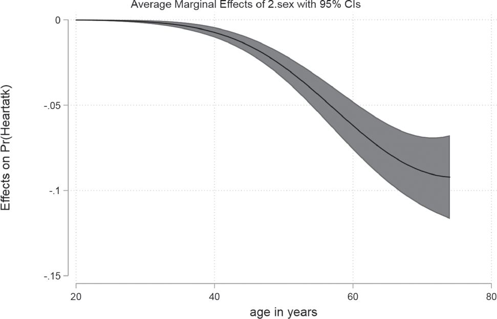
Remember that the AME tells you the marginal effect of changing gender, on the probability of having a heart attack. For example, in the graph above we see women with age 60 have a six percentage points lower probability of having a heart attack than men. We come to this conclusion, as the AME above is calculated for the 2.sex (see the title of the graph). As men are coded with zero and are, therefore, the category of reference, women are the second category, so the depicted effect shows the change from reference to this category. Additionally, a 95% confidence interval is included in the graph to improve the accuracy of your estimation.

One last option you can try is Marginal Effects at the Mean (MEM), which is just a combination of the aspects we have learned so far:

margins, dydx(sex) atmeans

The outcome tells us that when you had two otherwise-average individuals, one male, one female, the probability of having a heart attack would be 2.1 percentage points lower for the female.

8.3 Nested Models

What was explained on page 106 is also valid for logistic regressions: when you want to compare nested models make sure that they all use the same number of cases. You can use the AIC or the BIC to compare model fit (remember, lower values indicate better fitting models). Another option is the Likelihood-Ratio test, to see whether one model performs better than the other. To do this, estimate both models, save the results and run the test:

quietly logit heartatk c.age##c.age c.bmi i.region i.sex    //Run Model 1
estimates store Mfull                                       //Store results                       
quietly logit heartatk c.age if _est_Mfull                  //Run Model 2
estimate store Msimple                                      //Store results
lrtest Mfull Msimple

When you want to use point-and-click, go Statistics → Postestimation → Tests → Likelihood-ratio test.

When you receive a significant result, you can conclude that the extended model (the one with the largest number of variables) has a better model fit than the nested model.

Note that the order of the models in the lrtest command is not important, as Stata automatically recognizes which model is the one with the fewer variables used. Also keep in mind that you can use Average Marginal Effects to compare effects across models or samples, which is not possible with Odds or Logits (Mood, 2010).

8.4 Diagnostics

A review of the literature shows that there is no clear consensus about the diagnostics that are relevant for logistic regressions for yielding valid results. The following section is an overview of some aspects that will contribute to your model quality. The good news is that logistic regressions have lower standards than linear ones, so violations might not have too severe consequences. We will use the following model for all diagnostics shown here:

logit heartatk c.age##c.age c.bmi i.region i.sex

8.4.1 Model misspecification

You should create a model based upon your theoretical considerations. You can, statistically, further test whether your model has any missing or unnecessary variables included. To do so, run your model and type

linktest

or click Statistics → Postestimation → Tests → Specification link test for single-­equation models.

Stata produces a regression like output, with two variables, _hat and _hatsq. As long as the p-value of _hat is significant (p-value smaller than 0.05) and _hatsq is not significant (p-value larger than 0.05) your model specification should be fine. When _hat is not significant, your model is probably quite misspecified. When _hatsq is significant that means there are probably some important variables missing in your model. As you can see, our model should be OK.

8.4.3 Multicollinearity

Just like linear regressions, logistic ones are also influenced by a high correlation of independent variables. Testing this requires another user-written command (collin). Try

search collin

And look for the entry in the window that pops up (Figure 8.1). When the installation is complete, enter the command and the variables you used in the model:

collin age bmi region sex

:

As a general rule of thumb it might be a good idea to readjust your model when a variable shows a VIF above 10. In this case, remove one variable with a high VIF and run your model again. If the VIF is lower for the remaining variables, the choice might be a good idea.

8.4.4 Influential observations

Some observations might have uncommon constellations for values in their variables, which makes them influence results over-proportionally. It is usually a good idea to inspect these cases, although there is no general rule on how to deal with them. When you can exclude the possibility of plain coding errors, you can either keep or drop these cases. In contrast to the linear regression, we will use a slightly different measurement for influential observations in logistic regressions (Pregibon’s Beta, which is similar to Cook’s Distance). After your model was run type

predict beta, dbeta

or click Statistics → Postestimation → Predictions, residuals, etc. and select Delta-Beta influence statistic and give a name to the newly created variable, then click Submit. You will notice that only one variable was created, which we will inspect now. The total leverage of each case is summarized in this one. To detect outliers, use a scatterplot to assess the general distribution of the variable and scrutinize the problematic cases.

scatter beta sampl, mlabel(sampl)

:

We see a few extreme outliers, for example case 27,438. What is wrong here? Let’s have a closer look. We want to list all relevant values for this case, so we type

list heartatk sex age bmi region if sampl == 27438

:

The information here is perplexing. This woman with an age of 28 and a BMI of 27 (which counts as slightly overweight) reported a heart attack. Our common sense tells us that this is exceptional, as usually older men who are obese are prone to heart attacks. As this special case clearly violates the normal pattern, we could delete it and argue that this abnormal case influences our general results over-proportionally. Whatever you decide to do, report it in your paper and give a theoretical justification, as there is no general rule.

After you have excluded the case, run your model again and assess how the output changed.

logit heartatk c.age##c.age c.bmi i.region i.sex if sampl != 27438

- output omitted -