3. Variability: How Values Disperse

Chapter 2, “How Values Cluster Together,” went into some detail about measures of central tendency: the methods you can use to determine where on a scale of values you can find the value that’s the most typical and representative of a group. Intuitively, an average value is often the most interesting statistic, certainly more interesting than a number that tells you how values fail to come together. But understanding their variation gives context to the central tendency of the values.

For example, people tend to be more interested in the median value of houses in a neighborhood than they are in the range of those values. However, a statistic such as the range, which is one way to measure variability, puts an average into context. Suppose you know that the median price of a house in a given neighborhood is $250,000. You also know that the range of home prices—the difference between the highest and the lowest prices—in the same neighborhood is $300,000. You don’t know for sure, because you don’t know how skewed the distribution is, but a reasonable guess is that the prices range from $100,000 to $400,000.

That’s quite a spread in a single neighborhood. If you were told that the range of prices was $100,000, then the values might run from $200,000 to $300,000. In the former case, the neighborhood could include everything from little bungalows to McMansions. In the latter case, the houses are probably fairly similar in size and quality.

It’s not enough to know an average value. To give that average a meaning—that is, a context—you also need to know how the various members of a sample differ from its average.

Measuring Variability with the Range

Just as there are three primary ways to measure the central tendency in a frequency distribution, there’s more than one way to measure variability. Two of these methods, the standard deviation and the variance, are closely related and take up most of the discussion in this chapter.

A third way of measuring variability is the range: the maximum value in a set minus the minimum value. It’s usually helpful to know the range of the values in a frequency distribution, if only to guard against errors in data entry. For example, suppose you have a list in an Excel worksheet that contains the body temperatures, measured in Fahrenheit, of 100 men. If the calculated range, the maximum temperature minus the minimum temperature, is 888 degrees, you know pretty quickly that someone dropped a decimal point somewhere. Perhaps you entered 986 instead of 98.6.

The range as a statistic has some attributes that make it unsuitable for use in much statistical analysis. Nevertheless, in part because it’s much easier to calculate by hand than other measures of variability, the range can be useful.

The use of the range as the sole measure of variability in a data set has some drawbacks, but it’s a good idea to calculate it anyway to better understand the nature of your data. For example, Figure 3.1 shows a frequency distribution that can be sensibly described in part by using the range.

Figure 3.1. The distribution is approximately symmetric, and the range is a useful descriptor.

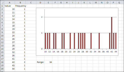
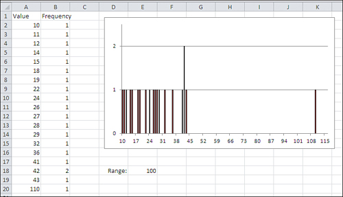
Because an appreciable number of the observations appear at each end of the distribution, it’s useful to know that the range that the values occupy is 34. Figure 3.2 presents a different picture. It takes only one extreme value for the range to present a misleading picture of the degree of variability in a data set.

Figure 3.2. The solitary value at the top of the distribution creates a range estimate that misdescribes the distribution.

The size of the range is entirely dependent on the values of the largest and the smallest values. The range does not change until and unless there’s a change in one or both of those values, the maximum and the minimum. All the other values in the frequency distribution could change and the range would remain the same. The other values could be distributed more homogeneously, or they could bunch up near one or two modes, and the range would still not change.

Furthermore, the size of the range depends heavily on the number of values in the frequency distribution. See Figure 3.3 for examples that compare the range with the standard deviation for samples of various sizes, drawn from a population where the standard deviation is 15.

Figure 3.3. Samples of sizes from 2 to 20 are shown in columns B through F, and statistics appear in rows 22 through 24.

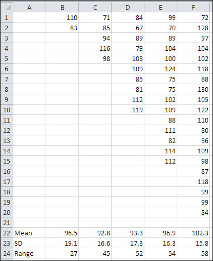
Notice that the mean and the standard deviation are relatively stable across five sample sizes, but the range more than doubles from 27 to 58 as the sample size grows from 2 to 20. That’s generally undesirable, particularly when you want to make inferences about a population on the basis of a sample. You would not want your estimate of the variability of values in a population to depend on the size of the sample that you take.

The effect that you see in Figure 3.3 is due to the fact that the likelihood of obtaining a relatively large or small value increases as the sample size increases. (This is true mainly of distributions such as the normal curve that contain many of their observations near the middle of the range.) Although the sample size has an effect on the calculated range, its effect on the standard deviation is much less pronounced because the standard deviation takes into account all the values in the sample, not just the extremes.

Excel has no RANGE() function. To get the range, you must use something such as the following, substituting the appropriate range address for the one shown:

=MAX(A2:A21) − MIN(A2:A21)

The Concept of a Standard Deviation

Suppose someone told you that you stand 19 units tall. What do you conclude from that information? Does that mean you’re tall? short? of average height? What percent of the population is taller than you are?

You don’t know, and you can’t know, because you don’t know how long a “unit” is. If a unit is four inches long, then you stand 76 inches, or 6′4″ (rather tall). If a unit is three inches long, then you stand 57 inches, or 4′9″ (rather short).

The problem is that there’s nothing standard about the word unit. (In fact, that’s one of the reasons it’s such a useful word.) Now suppose further that the mean height of all humans is 20 units. If you’re 19 units tall, you know that you’re shorter than average.

But how much shorter is one unit shorter? If, say, 3% of the population stands between 19 and 20 units, then you’re only a little shorter than average. Only 3% of the population stands between you and the average height.

If, instead, 34% of the population were between 19 and 20 units tall, then you’d be fairly short: Everyone who’s taller than the mean of 20, plus another 34% between 19 and 20 units, would be taller than you.

Suppose now that you know the mean height in the population is 20 units, and that 3% of the population is between 19 and 20 units tall. With that knowledge, with the context provided by knowing the mean height and the variability of height, “unit” becomes a standard. Now when someone tells you that you’re 19 units tall, you can apply your knowledge of the way that standard behaves, and immediately conclude that you’re a skosh shorter than average.

Arranging for a Standard

A standard deviation acts much like the fictitious unit described in the prior section. In any frequency distribution that follows a normal curve, these statements are true:

• You find about 34% of the records between the mean and one standard deviation from the mean.

• You find about 14% of the records between one and two standard deviations from the mean.

• You find about 2% of the records between two and three standard deviations from the mean.

These standards are displayed in Figure 3.4.

Figure 3.4. These proportions are found in all normal distributions.

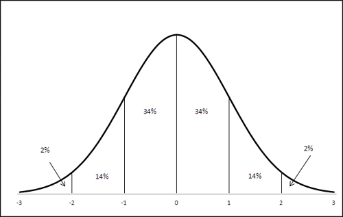
The numbers shown on the horizontal axis in Figure 3.4 are called z-scores. A z-score, or sometimes z-value, tells you how many standard deviations above or below the mean a record is. If someone tells you that your height in z-score units is +1.0, it’s the same as saying that your height is one standard deviation above the mean height.

Similarly, if your weight in z-scores is −2.0, your weight is two standard deviations below the mean weight.

Because of the way that z-scores slice up the frequency distribution, you know that a z-score of +1.0 means that 84% of the records lie below it: Your height of 1.0 z means that you are as tall as or taller than 84% of the other observations. That 84% comprises the 50% below the mean, plus the 34% between the mean and one standard deviation above the mean. Your weight, −2.0 z, means that you outweigh only 2% of the other observations. Hence the term standard deviation. It’s standard because it doesn’t matter whether you’re talking about height, weight, IQ, or the diameter of machined piston rings. If it’s a variable that’s normally distributed, then one standard deviation above the mean is equal to or greater than 84% of the other observations. Two standard deviations below the mean is equal to or less than 98% of the other observations.

It’s a deviation because it expresses a distance from the mean: a departure from the mean value. And it’s at this point in the discussion that we get back to the material in Chapter 2 regarding the mean, that it is the number that minimizes the sum of the squared deviations of the original values. More on that shortly, in “Dividing by N − 1,” but first it’s helpful to bring in a little more background.

Thinking in Terms of Standard Deviations

With some important exceptions, you are likely to find yourself thinking more about standard deviations than about other measures of variability. (Those exceptions begin to pile up when you start working with the analysis of variance and multiple regression, but those topics are a few chapters off.) The standard deviation is in the same unit of measurement as the variable you’re interested in. If you’re studying the distribution of miles per gallon of gasoline in a sample of cars, you might find that the standard deviation is four miles per gallon. The mean mileage of car brand A might be four mpg, or one standard deviation, greater than brand B’s mean mileage.

That’s very convenient and it’s one reason that standard deviations are so useful. It’s helpful to be able to think to yourself, “The mean height is 69 inches. The standard deviation is 3 inches.” The two statistics are in the same metric.

The variance is a different matter. It’s the square of the standard deviation, and it’s fundamental to statistical analysis, and you’ll see much more about the variance in this and subsequent chapters. But it doesn’t lend itself well to statements in English about the variability of a measure such as blood serum cholesterol or miles per gallon.

For example, it’s easy to get comfortable with statements such as “the mean was 20 miles per gallon and the standard deviation was 5 miles per gallon.” It’s a lot harder to feel comfortable with “the mean was 20 miles per gallon and the variance was 25 squared miles per gallon.” What does a “squared mile per gallon” even mean?

Fortunately, standard deviations are more intuitively informative. Suppose you have the mpg of ten Toyota cars in B2:B11, and the mpg of ten GM cars in B12:B21. One way to express the difference between the two brands’ mean gas mileage is this:

=(AVERAGE(B2:B11) − AVERAGE(B12:B21)) / STDEV(B2:B21)

That Excel formula gets the difference in the mean values for the two brands, and divides by the standard deviation of the mpg for all 20 cars. It’s shown in Figure 3.5.

Figure 3.5. The difference between two brands, expressed in standard deviation units.

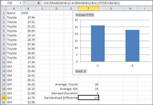
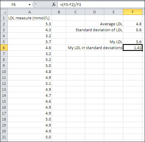
In Figure 3.5, the difference between the two brands in standard deviation units is 1.0. As you become more familiar and comfortable with standard deviations, you will find yourself automatically thinking things such as, “One standard deviation—that’s quite a bit.” Expressed in this way, you don’t need to know whether 26 mpg vs. 23 mpg is a large difference or a small one. Nor do you need to know whether 5.6 mmol/L (millimoles per liter) of LDL cholesterol is high, low, or typical (see Figure 3.6). All you need to know is that 5.6 is more than one standard deviation above the mean of 4.8 to conclude that it indicates moderate risk of diseases associated with the thickening of arterial walls.

Figure 3.6. The difference between one observation and a sample mean, expressed in standard deviation units.

The point is that when you’re thinking in terms of standard deviation units in an approximately normal distribution, you automatically know where a z-score is in the overall distribution. You know how far it is from another z-score. You know whether the difference between two means, expressed as z-scores, is large or small.

First, though, you have to calculate the standard deviation. Excel makes that very easy. There was a time when college students sat side by side at desks in laboratory basements, cranking out sums of squares on Burroughs adding machines with hand cranks. Now all that’s needed is to enter something like =STDEV(A2:A21).

Calculating the Standard Deviation and Variance

Excel provides you with no fewer than six functions to calculate the standard deviation of a set of values, and it’s pretty easy to get the standard deviation on a worksheet. If the values you’re concerned with are in cells A2:A21, you might enter this formula to get the standard deviation:

=STDEV(A2:A21)

(Other versions of the function are discussed later in this chapter, in the section titled “Excel’s Variability Functions.”)

The square of a standard deviation is called the variance. It’s another important measure of the variability in a set of values. Also, several functions in Excel return the variance of a set of values. One is VAR(). Again, other versions are discussed later in “Excel’s Variability Functions.” You enter a formula that uses the VAR() function just as you enter one that uses a standard deviation function:

=VAR(A2:A21)

That’s so simple and easy, it might not seem sensible to take the wraps off a somewhat intimidating formula. But looking at how the statistic is defined often helps understanding.

So, although most of this chapter has to do with standard deviations, it’s important to look more closely at the variance. Understanding one particular aspect of the variance makes it much easier to understand the standard deviation.

Here’s what’s often called the definitional formula of the variance:

Here’s the definitional formula in words:

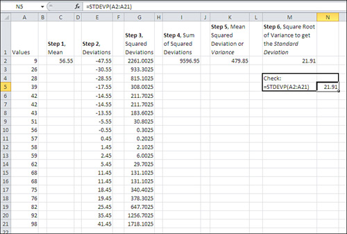
You have a sample of values, where the number of values is represented by N. The letter i is just an identifier that tells you which one of the N values you’re using as you work your way through the sample. With those values in hand, Excel’s standard deviation function takes the following steps. Refer to Figure 3.7 to see the steps as you might take them in a worksheet, if you wanted to treat Excel as the twenty-first-century equivalent of a Burroughs adding machine.

Figure 3.7. The long way around to the variance and the standard deviation.

1. Calculate the mean of the N values ). In Figure 3.7, the mean is shown in cell C2.
2. Subtract the mean from each of the N values . These differences (or deviations) appear in cells E2:E21 in Figure 3.7.
3. Square each deviation. See cells G2:G21.
4. Find the total (Σ) of the squared deviations, shown in cell I2.
5. Divide by N to find the mean squared deviation. See cell K2.

Step 5 results in the variance. If you think your way through those steps, you’ll see that the variance is the average squared deviation from the mean. As we’ve already seen, this quantity is not intuitively meaningful. You don’t say, for example, that John’s LDL measure is one variance higher than the mean. But the variance is an important and powerful statistic, and you’ll find that you grow more comfortable thinking about it as you work your way through subsequent chapters in this book.

If you wanted to take a sixth step in addition to the five listed above, you could take the square root of the variance. Step 6 results in the standard deviation, shown as 21.91 in cell M2 of Figure 3.7. The Excel formula is =SQRT(K2).

As a check, you find the same value of 21.91 in cell N5 of Figure 3.7. It’s much easier to enter the formula =STDEVP (A2:A21) than to go through all the manipulations in the six steps just given. Nevertheless, it’s a useful exercise to grind it out on the worksheet even just once, to help you learn and retain the concepts of squaring, summing, and averaging the deviations from the mean.

Figure 3.8 shows the frequency distribution from Figure 3.7 graphically.

Figure 3.8. The frequency distribution approximates but doesn’t duplicate a normal distribution.

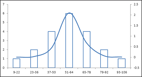
Notice in Figure 3.8 that the columns represent the count of records in different sets of values. A normal distribution is shown as a curve in the figure. The counts make it clear that this frequency distribution is close to a normal distribution; however, largely because the number of observations is so small, the frequencies depart somewhat from the frequencies that the normal distribution would cause you to expect.

Nevertheless, the standard deviation in this frequency distribution captures the values in categories that are roughly equivalent to the normal distribution.

For example, the mean of the distribution is 56.55 and the standard deviation is 21.91. Therefore, a z-score of −1.0 (that is, one standard deviation below the mean) represents a raw score of 34.64. Figure 3.4 says to expect that 34% of the observations will come between the mean and one standard deviation on each side of the mean.

If you examine the raw scores in cells A2:A21 in Figure 3.7, you’ll see that six of them fall between 34.64 and 56.65. Six is 30% of the 20 observations, and is a good approximation of the expected 34%.

Squaring the Deviations

Why square each deviation and then take the square root of their total? One primary reason is that if you simply take the average deviation, the result is always zero. Suppose you have three values: 8, 5, and 2. Their average value is 5. The deviations are 3, 0, and −3. The deviations total to zero, and therefore the mean of the deviations must equal zero. The same is true of any set of real numbers you might choose.

Because the total deviation is always zero, regardless of the values involved, it’s useless as an indicator of the amount of variability in a set of values. Therefore, each deviation is squared before totaling them. Because the square of any number is positive, you avoid the problem of always getting zero for the total of the deviations.

It is possible, of course, to use the absolute value of the deviations: that is, treat each deviation as a positive number. Then the sum of the deviations must be a positive number, just as is the sum of the squared deviations. And in fact there are some who argue that this figure, called the mean deviation, is a better way to calculate the variability in a set of values than the standard deviation.

But that argument, such as it is, goes well beyond the scope of this book. The standard deviation has long been the preferred method of measuring the amount of variability in a set of values.

Population Parameters and Sample Statistics

You normally use the word parameter for a number that describes a population and statistic for a number that describes a sample. So the mean of a population is a parameter, and the mean of a sample is a statistic.

This book tries to avoid using symbols where possible, but you’re going to come across them sooner or later—one of the places you’ll find them is Excel’s documentation. It’s traditional to use Greek letters for parameters that describe a population and to use Roman letters for statistics that describe a sample. So, you use the letter s to refer to the standard deviation of a sample and σ to refer to the standard deviation of a population.

With those conventions in mind—that is, Greek letters to represent population parameters and Roman letters to represent sample statistics—the equation that defines the variance for a sample that was given above should read differently for the variance of a population. The variance as a parameter is defined in this way:

The equation shown here is functionally identical to the equation for the sample variance given earlier. This equation uses the Greek σ, pronounced sigma. The lowercase σ is the symbol used in statistics to represent the standard deviation of a population, and σ² to represent the population variance.

The equation also uses the symbol μ. The Greek letter, pronounced mew, represents the population mean, whereas the symbol , pronounced X bar, represents the sample mean. (It’s usually, but not always, related Greek and Roman letters that represent the population parameter and the associated sample statistic.)

The symbol for the number of values, N, is not replaced. It is considered neither a statistic nor a parameter.

Dividing by N − 1

Another issue is involved with the formula that calculates the variance (and therefore the standard deviation). It stays involved when you want to estimate the variance of a population by means of the variance of a sample from that population. If you wondered why Chapter 2 went to such lengths to discuss the mean in terms of minimizing the sum of squared deviations, you’ll find the reason in this section.

Recall from Chapter 2 this property of the mean: if you calculate the deviation of each value in a sample from the mean of the sample, square the deviations and total them, then the result is smaller than it is if you use any number other than the mean. You can find this concept discussed at length in the section of Chapter 2 titled “Minimizing the Spread.”

Suppose now that you have a sample of 100 piston rings taken from a population of, say, 10,000 rings that your company has manufactured. You have a measure of the diameter of each ring in your sample, and you calculate the variance of the rings using the definitional formula:

You’ll get an accurate value for the variance in the sample, but that value is likely to underestimate the variance in the population of 10,000 rings. In turn, if you take the square root of the variance to obtain the standard deviation as an estimate of the population’s standard deviation, the underestimate comes along for the ride.

Samples involve error: in practice, their statistics are virtually never precisely equal to the parameters they’re meant to estimate. If you calculate the mean age of ten people in a statistics class that has 30 students, it is almost certain that the mean age of the ten student sample will be different from the mean age of the 30 student class.

Similarly, it is very likely that the mean piston ring diameter in your sample is different, even if only slightly, from the mean diameter of your population of 10,000 piston rings. Your sample mean is calculated on the basis of the 100 rings in your sample. Therefore, the result of the calculation

which uses the sample mean , is different from, and smaller than, the result of this calculation:

which uses the population mean μ.

The outcome is as demonstrated in Chapter 2.

Bear in mind that when you calculate deviations using the mean of the sample’s observations, you minimize the sum of the squared deviations from the sample mean. If you use any other number, such as the population mean, the result will be different from, and larger than, when you use the sample mean.

Therefore, any time you estimate the variance (or the standard deviation) of a population using the variance (or standard deviation) of a sample, your statistic is virtually certain to underestimate the size of the population parameter.

There would be no problem if your sample mean happened to be the same as the population mean, but in any meaningful situation that’s wildly unlikely to happen.

Is there some correction factor that can be used to compensate for the underestimate? Yes, there is. You would use this formula to accurately calculate the variance in a sample:

But if you want to estimate the value of the variance of the population from which you took your sample, you divide by N − 1:

The quantity (N − 1) in this formula is called the degrees of freedom.

Similarly, this formula is the definitional formula to estimate a population’s standard deviation on the basis of the observations in a sample (it’s just the square root of the sample estimate of the population variance):

If you look into the documentation for Excel’s variance functions, you’ll see that VAR() or, in Excel 2010, VAR.S() is recommended if you want to estimate a population variance from a sample. Those functions use the degrees of freedom in their denominators.

The functions VARP() and, in Excel 2010, VAR.P() are recommended if you are calculating the variance of a population by supplying the entire population’s values as the argument to the function. Equivalently, if you do have a sample from a population but do not intend to infer the population variance—that is, you just want to know the sample’s variance—you would use VARP() or VAR.P(). These functions use N, not the N − 1 degrees of freedom, in their denominators.

The same is true of STDEVP() and STDEV.P(). Use them to get the standard deviation of a population or of a sample when you don’t intend to infer the population’s standard deviation. Use STDEV() or STDEV.S() to infer a population standard deviation.

Bias in the Estimate

The main purpose of inferential statistics, the topic that’s discussed in the second half of this book, is to infer population parameters such as μ and σ from sample statistics such as and s. You will sometimes see and s and other statistics referred to as estimators, particularly in the context of inferring population values.

Estimators have several desirable characteristics, and one of them is unbiasedness. The absence of bias in a statistic that’s being used as an estimator is desirable. The mean is an unbiased estimator. No special adjustment is needed for to estimate μ accurately.

But when you use N, instead of the N − 1 degrees of freedom, in the calculation of the variance, you are biasing the statistic as an estimator. It is then biased negatively: it’s an underestimate of the variance in the population.

As discussed in the prior section, that’s the reason to use the degrees of freedom instead of the actual sample size when you infer the population variance from the sample variance. So doing removes the bias from the estimator.

It’s easy to conclude, then, that using N − 1 in the denominator of the standard deviation also removes its bias as an estimator of the population standard deviation. But it doesn’t. The square root of an unbiased estimator is not itself necessarily unbiased.

Much of the bias in the standard deviation is in fact removed by the use of the degrees of freedom instead of N in the denominator. But a little is left, and it’s usually regarded as negligible.

The larger the sample size, of course, the smaller the correction involved in using the degrees of freedom. With a sample of 100 values, the difference between dividing by 100 and dividing by 99 is quite small. With a sample of ten values, the difference between dividing by 10 and dividing by 9 can be meaningful.

Similarly, the degree of bias that remains in the standard deviation is very small when the degrees of freedom instead of the sample size is used in the denominator. The standard deviation remains a biased estimator, but the bias is only about 1% when the sample size is as small as 20, and the remaining bias becomes smaller yet as the sample size increases.

Degrees of Freedom

The concept of degrees of freedom is important to calculating variances and standard deviations. But as you move from descriptive statistics to inferential statistics, you encounter the concept more and more often. Any inferential analysis, from a simple t-test to a complicated multivariate linear regression, uses degrees of freedom (df) as part of the math and to help evaluate how reliable a result might be. The concept of degrees of freedom is also important for understanding standard deviations, as the prior section discussed.

Unfortunately, degrees of freedom is not a straightforward concept. It’s usual for people to take longer than they expect to become comfortable with it.

Fundamentally, degrees of freedom refers to the number of values that are free to vary. It is often true that one or more values in a set are constrained. The remaining values—the number of values in that set that are unconstrained—constitute the degrees of freedom.

Consider the mean of three values. Once you have calculated the mean and stick to it, it acts as a constraint. You can then set two of the three values to any two numbers you want, but the third value is constrained by the calculated mean.

Take 6, 8, and 10. Their mean is 8. Two of them are free to vary, and you could change 6 to 2 and 8 to 24. But because the mean acts as a constraint, the original 10 is constrained to become −2 if the mean of 8 is to be maintained.

When you calculate the deviation of each observation from the mean, you are imposing a constraint—the calculated mean—on the values in the sample. All of the observations but one (that is, N − 1 of the values) are free to vary, and with them the sum of the squared deviations. One of the observations is forced to take on a particular value, in order to retain the value of the mean.

In later chapters, particularly concerning the analysis of variance and linear regression, you will see that there are situations in which more constraints on a set of data exist, and therefore the number of degrees of freedom is fewer than the N − 1 value for the variances and standard deviations this chapter discusses.

Excel’s Variability Functions

The 2010 version of Excel reorganizes and renames several statistical functions. The aim is to name the functions according to a more consistent pattern, and to make a function’s purpose more apparent from its name.

Standard Deviation Functions

For example, Excel has since 1995 offered two functions that return the standard deviation:

• STDEV()—This function assumes that its argument list is a sample from a population, and therefore uses N − 1 in the denominator.

• STDEVP()—This function assumes that its argument list is the population, and therefore uses N in the denominator.

In its 2003 version, Excel added two more functions that return the standard deviation:

• STDEVA()—This function works like STDEV() except that it accepts alphabetic, text values in its argument list and also Boolean (TRUE or FALSE) values. Text values and FALSE values are treated as zeroes, and TRUE values are treated as ones.

• STDEVPA()—This function accepts text and Boolean values, just as does STDEVA(), but again it assumes that the argument list constitutes a population.

Microsoft decided that using P, for population, at the end of the function name STDEVP() was inconsistent because there was no STDEVS(). That would never do, and to remedy the situation, Excel 2010 includes two new standard deviation functions that append a letter to the function name in order to tell you whether it’s intended for use with a sample or on a population:

• STDEV.S()—This function works just like STDEV—it ignores Boolean values and text.

• STDEV.P()—This function works just like STDEVP—it also ignores Boolean values and text.

STDEV.S() and STDEV.P() are termed consistency functions because they introduce a new, more consistent naming convention than the earlier versions. Microsoft also states that their computation algorithms bring about more accurate results than is the case with STDEV() and STDEVP().

Excel 2010 continues to support the old STDEV() and STDEVP() functions, although it is not at present clear how long they will continue to be supported. In recognition of their deprecated status, STDEV() and STDEVP() occupy the bottom of the list of functions that appears in a pop-up window when you begin to type =STD in a worksheet cell. Excel 2010 refers to them as compatibility functions.

Variance Functions

Similar considerations apply to the worksheet functions that return the variance. The function’s name is used to indicate whether it is intended for a population or to infer a population value from a sample, and whether it can deal with nonnumeric values in its arguments.

• VAR() has been available in Excel since its earliest versions. It returns an unbiased estimate of a population variance based on values from a sample and uses degrees of freedom in the denominator. It is the square of STDEV().

• VARP() has been available in Excel for as long as VAR(). It returns the variance of a population and uses the number of records, not the degrees of freedom, in the denominator. It is the square of STDEVP().

• VARA() made its first appearance in Excel 2003. See the discussion of STDEVA(), earlier in this chapter, for the difference between VAR() and VARA().

• VARPA() also first appeared in Excel 2003 and takes the same approach to its nonnumeric arguments as does STDEVPA().

• VAR.S() is new in Excel 2010. Microsoft states that its computations are more accurate than are those used by VAR(). Its use and intent is the same as VAR().

• VAR.P() is new in Excel 2010. Its similarities to VARP() are analogous to those between VAR() and VAR.S().