About This Chapter
Control is a feedback system that covers both the action that implements the strategic decisions and the performance evaluation of personnel and operations. As a manager, you use feedback from financial performance reports that you normally receive at least monthly but possibly weekly, or even in real time. These reports may have different titles, but for your managerial responsibilities, the reports show the organization’s financial plan for a period, the actual performance achieved, and the difference between the two, which is called the variance.
You use the performance report specific to your responsibilities to identify activities that are not conforming to the organization’s plan and not contributing to its strategy. You conduct management by exception by investigating these differences between the plan and actual performance. The cost analysis helps you to determine your effectiveness and efficiency on implementing business strategies and to decide whether corrective action is necessary.
The two main techniques used to analyze departures from the plan are standard costing and budgetary control, which were discussed in the previous chapter. We looked at determining our strategic objectives and building those into financial plans to be used by managers. Once the plans have been established, control is maintained by comparing actual against planned performance. In this chapter, you will learn how to use the reports arising from the application of standard costing and budgetary control techniques to conduct an in-depth analysis of the performance reports you receive.
Any analysis benefits from detailed, accurate, and timely information. A thorough appraisal of standard cost variances can provide many benefits. However, the analysis is not completed by the mere calculation of differences between actual and planned performance but by an investigation as to why they arose and the decisions that need to be made that correspond with existing strategy or a reappraisal of that strategy.
One of the advantages of standard cost variances is that they are interrelated. You can calculate variances for a full range of activities, and the sum of these variances will demonstrate the impact of the variances on the planned profit. A hard financial number demonstrates strategic success or failure.
Depending on the nature of the organization, there are many variances that can be calculated. We are going to limit our discussions to two direct cost variances, two overhead variances, and a sales variance. These examples will explain the basic principles.
Direct Cost Variances
Direct Materials Variances
The direct material variances seek to answer the question whether the actual total cost of the direct materials for a certain level of production is the same as you planned. More importantly, you are guided to the probable reasons for any differences, and you can place these in a strategic context.
As explained in the previous chapter, the total cost of materials is made up by the amount of materials you use and the price you pay. Predetermined standards are set for both the usage level of direct materials for a given level of production and the price allowed per unit of direct materials.
The reason for the actual total cost of direct material differing from the plan is either we paid more or less per unit of materials than we planned or we used more or less materials than we planned. This could be due to poor planning, a change in market conditions that may require a new strategic approach, or a deviation from the original strategy.
The relationship between usage and price, and the formulas we use can be shown in a diagrammatic form:

This can be demonstrated by a simple example. A company is making leather luggage cases, and they set the following standards of materials for their “flight carry-on model”: 1.5 meters at $5.00 per meter. In 1 month, 500 cases were produced and the actual costs incurred were $3,496 for 760 meters of leather that were used in production. The calculations are as follows.
Total Direct Materials Variance:

Direct Material Price Variance:
(SP – AP)AQ
($5.00 – $4.60) × 760 = $304F
Material Usage Variance:
(SQ – AQ)SP
(750 – 760) × $5 = $50U
Just a note on the calculations before we explain the variances and their relationships: We were not given the actual price per meter of material, so we divided the total cost of $3,496 by the total usage of 760 meters to obtain the actual price per meter of $4.60. You will find that in a computerized system, all these calculations will be done, but it is useful for you to be able to understand the basis of the calculations.
Now let us look at the variances. As we have observed before, the variance is the difference between the standard and the actual. If your performance is better than the standard, you have a favorable variance. If it is worse than the standard, you have an unfavorable variance. When we use the term favorable and unfavorable, this refers to the impact of the actual performance on the planned profit.
In the formulas, we have a favorable total direct materials variance of $254F, and if there are no other variances with other direct costs, our actual profit for the period will be $254 higher than we planned. What we want to know is the reason for this improved performance, and the reasons are given in the two subvariances. We have a favorable price variance of $304 and $50 unfavorable for the usage variance. If you net these off, you get the overall favorable variance of $254.
Further investigation is required to explain these variances. One plausible reason is that an inferior quality material was purchased at a lower price than planned. However, this poor quality led to greater wastage and thus the unfavorable usage variance. There could, of course, be other reasons, but you will find it useful to relate the variable to each other and not only consider them in isolation.
In carrying out your investigations, it is essential to pay attention to the strategic context. Has the company decided on a cost reduction strategy, or is it aiming at producing a high-quality item. The overall material variance may be favorable when considered in isolation, but how do the individual components relate to the organization’s strategy?
In the previous example, we demonstrated the material usage variance: the actual quantity of materials used in the production of that number of cases. Some companies calculate a materials-purchased variance, as this is the responsibility of the purchasing manager, and the production manager is only responsible for the usage of the materials.
In calculating the direct labor variances, we use the same principles for material variances. Some companies will refer to this variance as the wage rate variance. As with materials, the reason for the actual total cost of direct labor differing from the plan is either we paid more or less per hour for labor than we planned or we required more or less labor hours than we had planned for that level of production.
The terms we use for the subvariances are direct labor rate—that is, how much we paid per hour—and direct labor efficiency variance (sometimes referred to as the labor productivity variance). This is the difference between the actual production achieved, measured in standard hours, and the actual hours worked, valued at the standard labor rate.
The relationship between these events and the formulas we use can be shown in a diagrammatic form:

We use the same example as before. A company is making leather luggage cases and has set the following labor standards for their “flight carry-on model.” Labor is expected to make two cases each hour, and the wage rate is $12 per hour.
In 1 month, 500 cases were produced, and the actual costs incurred were $11.50 per hour for 280 hours of work. The calculations are as follows:
Total Direct Labor Variance:
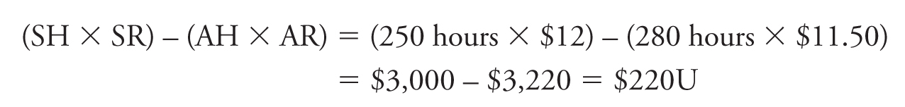
Labor Rate Variance:
(SR – AR)AH = ($12 × $11.50) 280 = $140F
Labor Efficiency Variance:
(SH – AH)SR = (250 – 280) × $12 = $360U
You can see that the unfavorable labor rate variance is explained by a favorable rate variance of $140F (we paid less per hour than planned) and an unfavorable efficiency variance of $360.
One plausible explanation is that we employed labor that was less skilled at a lower hourly rate, and therefore they took longer to do the work. Of course, you should always place any variance in the context of any related variance, in this case the materials used. On the face of it, inferior materials may have been used, so it is plausible that workers took longer because of the difficulty in working conditions with the poor quality materials.
The variances give you signposts to direct your investigations. If there are no variances, then you can practice “management by exception” and take no action. But remember that both favorable and unfavorable variances should be investigated. Toward the end of this chapter, we give advice on techniques that permit you to concentrate your attention where it is most needed.
Overhead Variances
In some companies, the standard costing system may be expanded to monitor and control indirect costs as well as direct costs. This is usually restricted to production overheads and is most useful where it is possible to analyze the budgeted and actual production overheads into their fixed and variable cost elements. You will realize that this aspect of variance analysis is closely linked to full or absorption costing where overheads are recovered. It also concentrates on activity levels and is therefore concerned with the utilization of capacity.
This area of analysis is frequently left to the accountant to investigate, as it relates to the budget setting for indirect costs and the decision on how they will be charged to production. In many organizations, the overhead cost is usually very significant and is a keystone of strategy formulation. It may be that in your career you will never encounter overhead variances but the following explanation provides a general foundation if you are taking a broader strategic perspective.
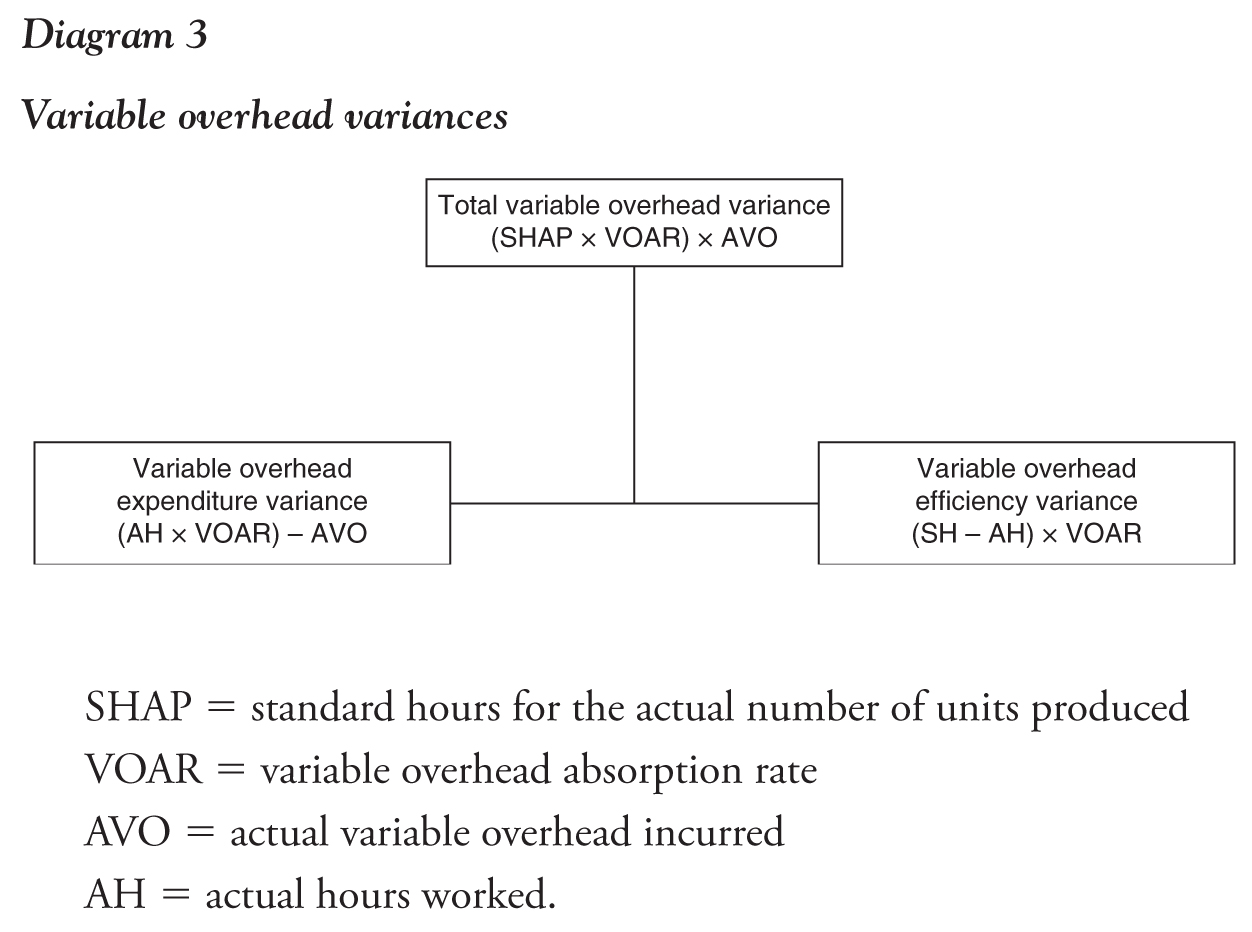
Variable Overhead Variances
We are continuing the principles established for the direct cost variances, but the terminology changes. A main variance is calculated and analyzed by two subvariances, as shown in the following diagram, assuming that the labor hour rate is used for charging overheads to production:
Example of Variable Overhead Variances
A company budgets its variable overheads for the period as $21,000, and it plans to produce 1,500 units with a standard labor time of 5 hours per unit. For the financial period, it produced 1,650 units. Its actual variable overhead cost is $20,000, and the actual hours worked were 8,500 hours.
The first stage is to calculate the standard hours allowed for the number of units actually produced (SHAP). This is 1,650 units × 5 hours per unit = 8,250 hours. The second calculation is the allocation rate that is based on labor hours. The standard labor hours are 1,500 × 5 = 7,500 hours. The predetermined allocation rate is therefore the budgeted overhead divided by the planned hours: $21,000/7,500 = $2.80.
Total Variable Overhead Variance:

Variable Overhead Expenditure Variance:

Variable Overhead Efficiency Variance:
(SHAP – AH) × VOAR = (8,250 – 8,500) $2.80 = 250 × $2.80 = $700U
After interpreting these calculations, we can see that the favorable total overhead variance of $3,100 favorable comprises two elements. The variable overhead expenditure variance shows that we only spent $20,000 on variable overheads, although the amount calculated for this level of production was $23,800. However, more labor hours were actually used than planned, and this resulted in an unfavorable variance of $700.
In looking at fixed overhead variances, you must bear in mind that we are assuming that these overheads will remain the same regardless of changes in activity. We are still going to be concerned whether the total amount of actual fixed overhead is the same as we planned. Efficiency is not an issue, but what is important is whether we used the capacity at our disposal to the extent that we planned, and this is known as the volume variance. In diagrammatic form, the variances are as follows:

Example of Fixed Overhead Variances
A company budgets its fixed overheads for the period as $16,500, and it plans to produce 1,500 units with a standard labor time of 5 hours per unit. For the financial period, it produced 1,650 units. Its actual fixed overhead cost is $15,000, and the actual hours worked were 8,500 hours. The calculation of standard hours from the actual number of units produced is 1,650 × 5 hours = 8,250 hours.
Assuming that we are using the labor hours as an allocation base for the fixed overhead, the calculation of the fixed overhead allocation rate is planned fixed overheads divided by planned labor hours. That is $16,500/7,500 = $2.20.
Total Fixed Overhead Variance:

Fixed Overhead Expenditure Variance:
(BFO – AFO) = ($16,500 – $15,000) = $1,500F
Fixed Overhead Volume Variance:
(SHAP × FOAR) – BFO = ($18,150 – $16,500) = $1,650F
The total fixed overhead is easy to understand if you remember full or absorption costing. At the beginning of the financial period, we calculated that we would charge $2.20 for every standard labor hour. The number of units produced (1,650) should have been completed in 8,250 labor hours. We therefore charged $18,150 for fixed overheads during the year, but as the actual overheads were only $15,000, we have a favorable variance of $3,150. One reason for this is that our actual fixed overheads were lower than our planned fixed overheads by $1,500—a favorable variance. Our fixed overhead volume variance of $1,650 favorable arises because we charged $18,150 to production for fixed overheads instead of the budget of $16,500 as our activity was higher than planned.
Sales Variances
Unfortunately, some companies pay too much attention to production cost variances and ignore sales variances. These are critical to the strategic management of any organization, and if you are in the sales function you need to understand these variances. There are several sales variances that can be calculated, such as sales price, sales volume, sales mix, sales quantity, market size, and market share variances.
In this section, we are going to concentrate on sales margin variances. However, you should be cautious in selecting the variances you need for your decision making and their interpretation. Using different bases for the calculation could give different results. The sales margin variance is widely used possibly because it generates variances that relate to the impact of the quantities sold and the prices charged. It is referred to as a sales margin variance, as it uses the profit margin in the calculations. The variances are as follows:

Example of Sales Margin Variance
A company establishes a standard selling price of $15 per unit for its product. The standard for the direct costs per unit is $4.40 and for production overheads $5.40 per unit. The total standard cost is therefore $9.80 to give a standard margin of $5.20. In the financial period, the company plans to sell 5,000 units of its main product. Ultimately, it actually sold 5,400 units at $14.00 per unit, and the actual cost was $9.00 per unit.
Total Sales Margin:
(ASV × ASM) – (SSV × SSM) = (5,400 × $5.00) – (5,000 × $5.20) = ($27,000 – $26,000) = $1,000F
Sales Margin Price Variance:
(ASM – SSM) × ASV = ($5.00 – $5.20) × 5,400 = $1.080A
Sales Margin Volume Variance:
(ASV – SSV) × SSM = (5,400 – 5,000) × $5.20 = $2080F
The analysis reveals that by reducing the selling price you get an adverse variance of $1,080. The reduction in the selling price and the change in actual costs results in a reduced sales margin of $5.00 per unit, but the significant increase in the volume sold gives a sales margin volume variance of $2,080F.
You will appreciate that, in using the sales margin, the relationship between the production costs and the selling price becomes critical. Although this example is simplified, it emphasizes that any strategic decisions on cost, volumes, and selling price cannot be made without the relevant data. Standard costing provides that information.
Budget Variances
Identifying Variances
As you might expect, the actual performance of an organization will not correspond entirely with the original budgets as the year progresses. As with standard costing, there will be differences between planned and actual performance. Where the actual cost differs from the budget, there will be either an adverse or an unfavorable variance. Where the actual costs are lower than the budget, there will be a favorable variance. With sales, the reverse is true. If actual sales are higher than the budget, the variance is favorable; if lower, the variance is adverse.
Similar to standard costing, a budget is determined to be unfavorable or favorable due to its impact on the budgeted profit. If your actual costs are $10,000 higher than planned costs, this will mean that your budget profit is hit by the $10,000. If your sales are $5,000 lower than planned, then your actual profit will be unfavorably affected compared to your budget.
Unlike standard costing, we do not have a hierarchy of formulas to assist us in our investigations, so you must be able to appreciate the relationship of the variances. As a manager, you will normally receive a budget report monthly comparing your department’s actual performance against the budget. The report you receive will most likely be a “line-by-line” budget and will show the planned amount for the month, the actual, and the variance. Some reports may also show the same information for the year to date.
Table 4.1 shows the performance for 1 month. This budget report has only seven lines of information, and you can expect to see budgets with many more items identified.
We do not know whether this is a merchandising company that buys goods from suppliers and then sells them, or if it is a manufacturer. It does not matter! The key message when looking at this budget is that the month was a disaster. We budgeted for a profit of $50,000, but the actual profit was only $10,000 due to aggregate variances of $40,000 unfavorable. If the company has a strategy, it needs urgent treatment before it expires completely.
As a manager, it will be your responsibility to identify the main issues and to take action. To do this, you will need to identify which are the important variances, and “management by exception” is widely used. In other words, you investigate those variances that are exceptional, usually because of their size. However, this is not the only way.
In the next section, we will explain a more sophisticated approach than just using monthly “dollar” size as a measure. But first, let us improve the budget report in Table 4.1 to make it more helpful. One adjustment is to add a line to show “gross profit.” This is the difference between the cost to you of the goods you sell or manufacture and the price you receive for them. It is a key indicator of performance.
Table 4.1 Monthly budget

The second adjustment will be to add a final column to show the percentage impact of the variance. We have calculated the figures by expressing the variance as a percentage of the budget. Some organizations prefer to use the actual, and some will calculate the variance as a percentage of the budgeted or actual profit. You need to ascertain the practice in your own organization. The adjusted report is shown in Table 4.2.
One figure still missing is the quantity of items sold, and we will examine the value of this information when we consider flexible budgets in the next chapter.
Before looking more closely at some of these figures, let us tackle the easier items. A saving of $15,000 (12.5 percent) is made on salaries. If you are a good manager, you should already know the events that led to this and made the appropriate decisions.
Administration overheads show a substantial unfavorable variance in both the dollar amount and the percentage. Once again, you should be already aware of the background. One possible scenario is that you are unable to hire full-time employees and resort to outsourcing or other support mechanisms, which is coded into the administration overheads. Check on this!
The most intriguing combination of variances revolves around the revenue and cost of sales figures. Although the variances are not large, you should always be alert to changes that directly affect gross profit. As the percentage gross profit has declined, this suggests several different scenarios, two of which are typical:
Table 4.2 Adjusted monthly budget report

1.Your costs have increased, so you have increased your selling price but insufficiently to maintain your gross margin.
2.You have reduced your selling price, and your volume of sales has increased, but this increase in volume has led to higher cost of goods sold.
The substantial increase in selling overheads indicates a push on sales, but the saving on distribution costs suggests that there has not been an increase in volume. These are intriguing questions, and all of them reflect the financial implications of the strategies that you have pursued during the month.
In this simple example, we have only been able to speculate on reasons for the variances, and as a manager you should be so familiar with the activities for which you have a responsibility that you know where to carry out your investigations. So the variances are operating as signposts, but with a much more comprehensive budget, you need some guidelines to know how to apply “management by exception.” We discuss this in the next section.
Investigating Variances
As a manager, you should be monitoring activities in your department and identifying where things are going well or poorly. Both favorable and unfavorable variances should be investigated. The budget report will give you the financial consequences of these occurrences and also illuminate some aspects that would not otherwise be apparent. It also allows you to concentrate your attention on where the financial impact is important. There are several ways to identify the variances you should investigate.
Dollars and Percentages
One way to measure the importance of the variance is to set limits on the differences and any variance outside the limit of your investigation. You might set as a general rule that any variance $20,000 over or under the budgeted figure will be investigated. If we apply this rule to the previous example, only the selling overheads will be investigated. Similarly, if we use only percentages, we would miss important issues. The way to resolve this dilemma is to use both dollars and percentages. You would therefore investigate any variance that deviated by either $20,000 or 10 percent.
Even that could result in some important areas of missing investigation, so we will explain how you can improve your analytical abilities.
Recurring Variances
Variances may fall within the boundaries you have set, so on a month-by-month basis you may not feel concerned. What you must be alert to is the situation where a variance is occurring repeatedly for the same item. Based on the data in Table 4.2, we give the first 3 months’ variances for distribution costs in Table 4.3.
Although the variance for each month falls within our limits, it is worrying that each month shows a variance. This is a favorable variance and in dollars. We are not looking at substantial amounts, but the percentage is hovering close to our 10 percent time after time. It would be worth looking at this variance to ascertain the reason.
Table 4.3 Monthly variances: Distribution costs

The first move would be to look at the original budget and to see whether it appears credible, particularly as the organization may have increased its sales volume. You will often find that in your investigations you need to consider the entire strategic demands of the entire activity. If the budget seems credible, the next question may be whether new and more efficient procedures have been introduced. If so, let us see whether we can improve them further or apply them in other parts of the organization.
If, after pursuing the above lines of inquiry and any others you can identify, there is no obvious answer, a deeper delve may be necessary. We mentioned in the previous chapter about the relationships between budgets and behavior. Some managers like to “beat their budgets” and may find devious ways to do so. Ignoring maintenance, losing invoices, using inferior materials, and infringing regulations are just some of the ways. As a manager you would have to consider the possibility that subordinates may be adopting unacceptable practices.
Trends
In this example, we are going to apply our limits of $20,000 and 10 percent again but use new data. Let us assume that for maintenance costs in the factory, the variances for 3 months are as shown in Table 4.4.
Although comfortably under our budget limits, this variance is increasing each month. You do not want this to blow up in your face sometime in June or even earlier. If you see the trend of a variance increasing or decreasing over a period of time, you need to investigate.
Table 4.4 Monthly variance


Figure 4.1. Visual control chart
Control Charts
The degree of sophistication you apply to these can differ from the visual to the statistical. As a busy manager, you sometimes need to focus on a few key budget figures. You may find it useful to show these in a chart form and plot the data over a period of time. This can be useful on your office wall or can form part of a presentation. The example in Figure 4.1 plots the variance for the total departmental costs over a 6-month period.
In Figure 4.1, it appears as if the manager reversed an unfavorable January and established increasingly favorable variances until March. Performance then commenced to June when it again entered the unfavorable zone. The reasons for this unfavorable variance need to be investigated. The manager could also add lines to indicate where investigations should commence or plot the standard deviations.
Contradictions and Anomalies
The final method suggested is easier for the experienced manager, but all managers should be thinking along these lines, with the feeling that “something is not right” when you look at your monthly budget report. Possibly you know that certain costs have increased, but an unfavorable variance against budget is not being shown. Why not? You may have introduced more efficient processes and procedures, but a favorable variance is not being shown. Why not?
In some instances, it is the relationship between various activities as reflected in the budgets that generates a contradiction. In Figure 4.1, the sales revenue increased. We do not know whether that was an increase due to price or volume, but if it is the latter, you would have expected the distribution costs to also increase.
In this section, we looked at the variances arising from comparing the actual performance against the static or fixed budget. Several of our comments are based on the fact that the static budget is set at the beginning of the financial period, and no changes are made to it during the period. For an organization in a stable environment, this is a good approach because it gives certainty and a clear direction toward the strategic objectives.
But what if the environment changes during the financial period, and there are variations in activity? You would expect the actual performance to be different from the static budget. This difficulty is resolved by the flexible budget that we explain in our next section.
Flexible Budgets
Fluctuating Activity
The discussions in the preceding section concerned static, or fixed, budgets. These are set at the beginning of the year and are not changed merely because the actual activity levels differ from the budget activity. If there are significant changes in the environment, or the organization amends its strategic plan, changes may then be made. Static budgets are appropriate where activity levels are consistent or are controllable by the manager.
A major drawback of static budgets is that an unfavorable variance can arise in variable cost variances because of a beneficial increase in activity levels. For example, actual sales volume may be higher than planned because of a buoyant market. This growth in sales volume will cause an increase in actual production and distribution costs to support the sales. With a fixed budget, these will show as unfavorable variances although the overall organizational performance is good.
This problem can be resolved by using a flexible budget where activity levels fluctuate and are uncontrollable by the manager responsible. The flexing of the budget refers only to variable costs and if there is a cost variance it can be assumed to be due to an increase or decrease in activity.
The Flexed Budget
The usual procedure is to set the budget at the beginning of the period for the planned level of activity. At the end of the month, the variable costs in the budget are then adjusted in line with the actual level of activity achieved. Fixed costs are not normally flexed as they should remain the same regardless of any changes in activity within the relevant range.
In Table 4.5, we compare a static and flexible budget. The static budget was set for 40,000 units to be produced and sold. At the end of the month, the actual number of units produced and sold is 45,000. The static budget is then flexed, and the results are shown in the next column. The actual performance is then compared with the flexed budget to give the variance in the final column.
The calculation of the flexed budget is the total budgeted sales or cost amount divided by the budgeted number of units. The resulting budgeted amount per unit is then multiplied by the actual number of units for the financial period.
First, a comment on the revenue. For the same number of units, we managed to obtain $3,000 more than the flexible budget. So our volume increased, but our total actual sales is higher than our flexed budget. This suggests that there has been a small price increase. This could have been a strategic decision or merely an opportunistic action.
Next, the variable costs. If we had compared our actual variable costs to the original static budget, all items would have shown an unfavorable variance because production was higher than originally planned. Comparing to our flexible budget, we see that only direct materials give an unfavorable variance. The variance is not large, but it may be worth investigating. One plausible reason may be that a better quality of material was used, and this may also explain the slight increase in the selling price. Once again, the question arises whether this is in line with the strategy.
Table 4.5 Static and flexible budgets compared

Fixed overheads should have remained the same, but the one to investigate is insurance. It is possible that the original quote was not correct, or additional items were insured that were not in the original quote.
The aforementioned example suggests that flexible budgeting is far superior, as it results in more credible budgets. However, there are disadvantages. The production manager has planned originally to manufacture 200,000 units but is called upon to increase this by 25,000 units. This means more materials have to be ordered, more labor may be required, and there may not be sufficient capacity on the machinery, so overtime has to be worked. In other words, the planned coordination of activities can be disrupted. If there is a strong strategy underpinning these actions, there is no problem, and proper coordination of all the activities should have been achieved.
There is also a problem if actual activity levels are lower than planned. As the variable costs will be flexed, there may be no unfavorable variances. The managers in those departments may be very satisfied with the performance of their own areas of responsibility, but at the organizational level it may be a disaster. Managers are not only individually responsible for their own areas but are also collectively responsible for the organizational performance and adherence to the strategy. Flexible budgets may distract from that collective approach to achieving the strategic goals.
Budgeting Assessed
The Strengths
In the previous chapter, we explained the relationship between strategic objectives and budgeting and described budgeting procedures, the interrelationships of budgeting, and the use of budgets as monitoring and control mechanisms. Budgetary control has many strengths, and there are potential advantages to an organization using the technique:
•The strategic goals of the organization are translated into detailed financial plans.
•A coherent system of monitoring and control is established.
•The identification of budget centers structures the responsibilities of managers for identified activities.
•Integration of the various parts of the organization takes place.
•Managers are motivated by the clarification of objectives, the performance expected, and the reporting of progress.
•The analysis of variances allows managers to take timely corrective action wherever necessary.
•Where actual activity fluctuates, flexible budgets provide a method for relating variable costs to these changes.
Although budgetary control is widely used, there are some potential drawbacks even with a well-managed system:
•Establishing budgets is a time-consuming process.
•If static budgets are used and activity fluctuates, the reported variances will have no credibility.
•Managers can become demotivated if they consider the budgets are unrealistic.
•Once managers realize that they will meet their budget amounts, there is little incentive to work harder.
•The system may encourage dysfunctional work behavior, as discussed in the previous chapter.
•It is a complex process requiring skills in both setting plans and implementing them in the organization.
•Budgets emphasize central control that may inhibit managerial initiative.
•In a turbulent environment, the assumption that the long-term future can be predicted and activities driven by these plans may not be viable.
Conclusions
In this chapter, we demonstrated how you can monitor and control actual performance. This is achieved by comparing your actual performance against your standards or budgets for the financial period and investigating the variances. If you performed better than planned, you will have a favorable variance; if worse than planned, an unfavorable variance.
The first part of the chapter examined standard cost variances. The basic principle underpinned all the calculations, and we demonstrated
•using material price variance to investigate differences due to the actual price for materials being different from the plan
•using material usage variance to investigate differences due to the actual quantity of materials used in production being different from the plan
•using labor rate variance to investigate differences due to the actual rate paid to labor being different from the plan
•using labor efficiency variance to investigate differences due to more or less work completed than was allowed for in the planned time
We also explained overhead expenditure variance and the overhead volume variance, although these are usually of greater interest to the accountant than the general manager. Sales margin variances were also explained, and these can be of critical importance. You need to take care in defining and interpreting this variance.
With budget variances, we explained how to identify the variances and gave the following guidelines to determine which variances you need to investigate:
•Dollar amounts or percentage guidelines can be set so that you investigate any variance outside these boundaries.
•Recurring variances may not be large, but if they continue month after month, they should be investigated.
•Trends, either favorable or unfavorable, should be watched. If a variance is gradually increasing or decreasing month after month, you should examine it in order to avoid a future problem.
•Contradictions and anomalies are likely to arise, and as a manager, you should be alert to any variances that do not match your personal observations or your experience.
Budgetary control is a time-consuming process, and we completed the chapter by reflecting on its strengths and weaknesses. We also discussed the criticisms made of the technique. Despite the issues concerning the application and maintenance of the system, few companies would abandon it completely, as it is so entwined with corporate strategy. The explanations and guidance in this chapter may assist in you ensuring that you gain the maximum benefits from the technique.