
3. Demand Planning
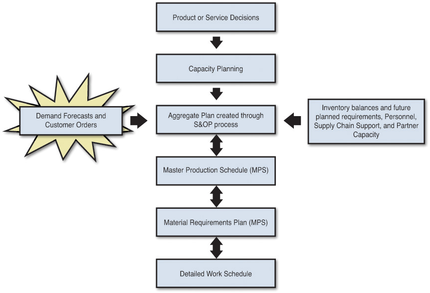
It’s only been in the past 20 years or so that businesses have truly come to realize the importance of forecasting. If you think about it, forecasting is usually the first step in the planning and scheduling process for most goods and service organizations, and forecasts for demand drive everything in an organization: from longer-term decisions (3+ years out) as to new facilities and products, to medium-term decisions (months to years out) such as production planning and budgeting, and the short-term (months to a year at most), where we need to know what to produce (or purchase) and deploy (see Figure 3.1).
The function itself has evolved from being an almost “dreaded” responsibility of sales and marketing, to where operations took control to produce stable production requirements, and on to today where it is most typically part of the supply chain function, where it can rise to the level of importance in an organization to the point where there may be a director of forecasting or demand planning. In fact, there is now a professional organization dedicated to the profession: the Institute of Business Forecasting & Planning (www.ibf.org).
Forecasting Used to Be Strictly Like “Driving Ahead, Looking in the Rearview Mirror”
Historically, manufacturers forecasted sales based on shipments to customers only, which was less than optimal because 1) what we sold may not have been what was ordered (or where it was supposed to ship from) and 2) the true driver of most businesses and services is the consumer, not necessarily our distribution channels.
These limitations were due primarily to companies working in more of a “vacuum” because data was hard to get and limited to internal sources and storage space expensive and limited.
Many companies also operated under a two-number system, where sales and marketing budgeted one number (which might be changed only once per quarter) and manufacturing developed their own SKU (stock keeping unit) forecast based on more current sales. In some cases, there was even a third number used by those responsible for finished goods deployment to distribution centers, which in many cases was based on percentage allocations of one of the two aforementioned national or global forecasts.
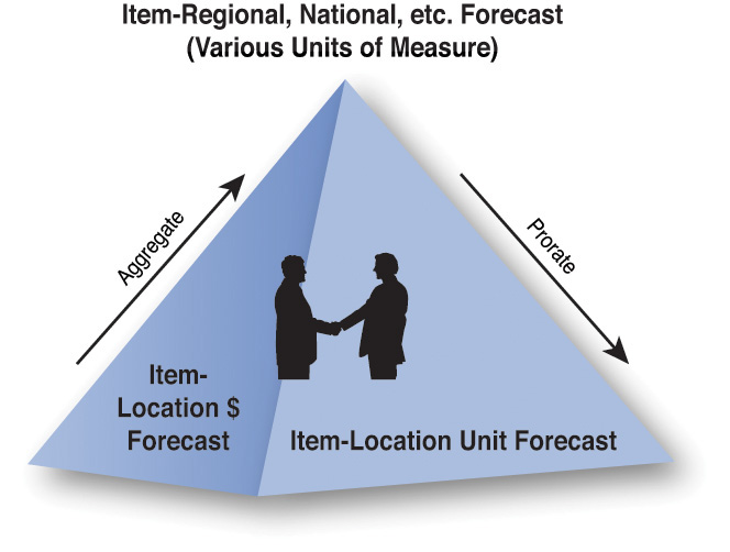
As technology became more readily available (and more affordable) in the mid-1980s to early 1990s, many businesses were able to begin to get a better handle on the forecasting process. Using the pyramid approach to forecasting (see Figure 3.2), organizations were able to develop a bottom up/top down one-number forecast, which used various statistical methods as well as other sources of information at various levels of detail. These one-number forecasts were able to drive budgeting, production, and deployment simultaneously and be updated typically on a monthly (or more often basis).
The availability and sharing of point-of-sale (POS) data from either paid services or larger customers was also integrated into the process using collaborative programs between manufacturers and retailers such as quick response and efficient consumer response (to be discussed in more detail later) to help reduce the bullwhip effect.
Forecasting Realities
You need to understand certain realities about forecasting before getting into the details of the process:
![]() All forecasts are wrong. It’s rare that a forecast is 100% accurate. The idea is to have an integrated, collaborative process that minimizes variance of actual versus target. You’ll learn later in this book about the process and importance of setting and measuring forecast accuracy targets.
All forecasts are wrong. It’s rare that a forecast is 100% accurate. The idea is to have an integrated, collaborative process that minimizes variance of actual versus target. You’ll learn later in this book about the process and importance of setting and measuring forecast accuracy targets.
![]() The more “granular” the forecast, the less accurate it is. A national forecast for a family of items is likely to be more accurate than a weekly forecast for an SKU at a distribution center that handles a region of the country. We can compensate for some of the inaccuracy through proper inventory planning, factoring in scientific safety stock inventory based on desired service levels and reduced lot sizes and cycle times included in Lean, as covered later in the book.
The more “granular” the forecast, the less accurate it is. A national forecast for a family of items is likely to be more accurate than a weekly forecast for an SKU at a distribution center that handles a region of the country. We can compensate for some of the inaccuracy through proper inventory planning, factoring in scientific safety stock inventory based on desired service levels and reduced lot sizes and cycle times included in Lean, as covered later in the book.
![]() It’s easier to forecast next month more accurately than next year. If we know what we sold yesterday, we typically have a better idea of what we’ll sell today; whereas 12 months from now, a lot of things can happen that can affect sales.
It’s easier to forecast next month more accurately than next year. If we know what we sold yesterday, we typically have a better idea of what we’ll sell today; whereas 12 months from now, a lot of things can happen that can affect sales.
![]() You will get a more accurate forecast using demand history rather than sales history. Years ago, when data storage costs were high and capacity lower, most companies only stored sales information. Today, most store order or demand information as well. Unless your company has a 100% service level, there will be occasions where you ship short, late, or from the “wrong” location. If you only use sales history, you would be forecasting to repeat yesterday’s failure. That’s why you should always use demand history to drive statistical forecasts.
You will get a more accurate forecast using demand history rather than sales history. Years ago, when data storage costs were high and capacity lower, most companies only stored sales information. Today, most store order or demand information as well. Unless your company has a 100% service level, there will be occasions where you ship short, late, or from the “wrong” location. If you only use sales history, you would be forecasting to repeat yesterday’s failure. That’s why you should always use demand history to drive statistical forecasts.
![]() Forecasting really is a blend of art and science. As we will discuss, there are both qualitative and quantitative methods of forecasting. Today, the best practice is a combination of both, in addition to collaboration with supply chain partners, providing better visibility downstream in the demand chain.
Forecasting really is a blend of art and science. As we will discuss, there are both qualitative and quantitative methods of forecasting. Today, the best practice is a combination of both, in addition to collaboration with supply chain partners, providing better visibility downstream in the demand chain.
Types of Forecasts
Organizations have various forecasting needs. The major ones are as follows:
![]() Marketing requires forecasts to determine which new products or services to introduce or discontinue, which markets to enter or exit, and which products to promote.
Marketing requires forecasts to determine which new products or services to introduce or discontinue, which markets to enter or exit, and which products to promote.
![]() Salespeople use forecasts to make sales plans, because sales quotas are generally based on estimates of future sales.
Salespeople use forecasts to make sales plans, because sales quotas are generally based on estimates of future sales.
![]() Supply chain managers use forecasts to make production, procurement, and logistical plans.
Supply chain managers use forecasts to make production, procurement, and logistical plans.
![]() Finance and accounting use forecasts to make financial plans (budgeting, capital expenditures, and so on). They also use them to report to Wall Street with regard to their earnings expectations.
Finance and accounting use forecasts to make financial plans (budgeting, capital expenditures, and so on). They also use them to report to Wall Street with regard to their earnings expectations.
Demand Drivers
In general, demand can be driven by a number of internal and external factors, which need to be identified and understood.
Internal Demand Drivers
These types of drivers of demand include sales force incentives, consumer promotions, and discounts to trade. It was only in the past 20 years that some manufacturers and retailers began to better understand the full impact of these drivers on the supply chain resulting in the bullwhip effect.
For example, Procter and Gamble and Walmart have partnered in everyday low pricing (EDLP) to reduce costs and improve service. At one point, P&G went as far as stationing 200 employees at Walmart’s headquarters in Bentonville, Arkansas.
Previously, supply chain and operations were at the mercy of these internal drivers and had to live through the consequences. Of course, they will always exist to some degree.
External Demand Drivers
These drivers, although not controllable to any great degree, can be managed better through best practice techniques with a structured methodology in place that employs improved communications and integration with other departments within an organization and with customers. These can include events in the environment that are mostly unpredictable, such as terror attacks and stock market crashes, and others that are due to a lack of good communication and visibility, such as new distribution and larger-than-anticipated orders.
Forecasting Process Steps
Everyone does things a little different, so it’s always a good idea to develop a standard methodology for a process. In the case of demand forecasting, certain general steps should be included (Heizer & Render, 2013):
1. Determine the use of the forecast. Varies by industry and company. In the case of manufacturing, it may be to drive production and deployment, in the case of retail it might be to determine purchasing requirements and for pure service companies might be used primarily for labor staffing.
2. Select the items to be forecasted. Will we be forecasting by individual item in various granulations, and at what levels and units of measure will be need to be able to aggregate forecasts and demand history?
3. Determine the time horizon of the forecast. Do we need to look at it in the short, medium, or long term (or all of the above), and what type of time planning buckets are appropriate (for example, 30 days or less: daily buckets; 1–3 months out: weekly buckets; and 4+ months: quarterly buckets).
4. Select the forecasting model(s) and methods. Based on a number of things we will be discussing, such as where a product is in its lifecycle, will we use qualitative, quantitative, or a blend of models? To what degree will we integrate externally supplied information (for example, customer forecasts, POS data, CPFR, and so on), and what weight will we give it?
5. Gather the data needed to make the forecas. When using forecasting software, the initial integration will consider much of this, such as using demand versus sales, as mentioned previously, eliminating data errors, and so on. Once this integration has been created and data validated, it becomes more of a maintenance issue for things such as new and discontinued items.
6. Generate forecasts. Typically, statistical methods are used to generate a baseline forecast, possibly at different levels of detail. The planner will then usually audit the results and, if needed, try other statistical models. They will then factor in management overrides based on their experience and knowledge as well as promotional plans, sales estimates, and externally supplied information mentioned earlier.
7. Validate and implement the results. During the demand part of the sales and operations planning (S&OP) process that we will discuss in the next chapter, forecasts are reviewed by cross-functional teams at various levels of detail and units of measure to ensure the highest level of accuracy possible. This will ultimately lead to a one-number system that was discussed earlier so that everyone is on the same page.
During this time, recent forecast accuracy will be evaluated, as well, to help target improvement. It is also during this step that the new forecasts are saved to be measured later for accuracy against predetermined variance/error targets, as discussed later in the chapter.
Many companies cycle through this process on a monthly basis (this again varies by industry and how the forecasts will be used), but forecasts are typically adjusted on an as-needed basis due to over/undersells, new demand information, changes to promotions and discounts, and so on.
Quantitative Versus Qualitative Models
There are two general types of forecasting models: quantitative and qualitative.
Qualitative Models
The qualitative method is typically used when the situation is somewhat vague and there is little data that exists. It is useful for creating forecast estimates for new products, services, and technology. Generally, it relies heavily upon intuition and experience.
Qualitative methods include knowledge of products, market surveys, jury of executive opinion, and the Delphi method.
Knowledge and Intuition of the Products
A forecast can come from the experience of a planner/forecaster who has years of experience with the product and can look over historical and forecast statistical estimates to make adjustments based on his or her judgment. This same method can be used with other people in the organization such as sales and marketing to gather their estimates.
However, you must always be aware of biases that may result from different individual’s motivation. For example, sale personnel may have an incentive to hit a high target to reach a bonus.
In my experience as a senior forecaster at Unilever, after awhile I was able to determine that sales estimates were typically 50% high, and once factoring that in, they were fairly useful (at least to start a dialogue). It is also important to be able to share forecast and historical data in units of measure and levels of aggregation that are meaningful to others. For example, the sales department thinks more in terms of revenue dollars, customers, and product categories. So, a good forecasting process and software system should be able to convert data back and forth to both present the data and receive feedback.
Market Surveys
Market surveys involve the process of gathering information from actual or potential customers. I’m sure most of us have experienced being asked to answer a survey in a mall. When I was an employee at Burger King Corporation at their headquarters in Miami, Florida, we would be asked on occasion to visit the test kitchen upstairs. We would then try different versions of current and new/test items. Usually we were asked to compare items that might have subtle differences, like different brands of ketchup.
Another example are focus groups where people are asked about their perceptions, opinions, beliefs, and attitudes toward a product, service, concept, advertisement, idea, or packaging. Questions are sometimes asked in a group setting, and participants can talk with other group members.
Jury of Executive Opinion
In the jury of executive opinion forecasting method, managers within the organization get together to discuss their opinions on what sales will be in the future. These discussion sessions usually resolve around experienced guesses. The resulting forecast is a blend of informed opinions, with some use of statistical methods.
Delphi Method
In the Delphi method, which is a bit more formal than the jury of executive opinion method, the results of questionnaires are sent to a panel of experts. Through an iterative process, multiple rounds of questionnaires are sent out, and the anonymous responses are aggregated and shared with the group at the end of each round. The experts are allowed to modify their answers for each round. The Delphi method seeks to reach the correct response through consensus.
Both the Delphi and jury of executive opinion forecasting methods are usually a bit more strategic in nature and used more in developing higher-level longer-terms forecasts.
Quantitative Models
As opposed to qualitative methods, quantitative methods are typically used when the situation is fairly stable and historical data exist. As a result, it is used primarily for existing/current technology products and involves a variety of mathematical techniques we cover in some detail later in this chapter under the two major categories of time series and causal models.
Time Series Models
Time series forecasting uses a set of evenly spaced numeric data that is obtained by observing response variable at regular time periods. The forecasts are based on past values and assume that factors influencing past, present, and future will continue. Relatively simple and inexpensive methods such as moving averages and weighted moving averages are used to predict the future.
Associative Models
Associative (often called causal) models forecast based on the assumption that the variable to be forecast (that is, dependent) has a cause-and-effect relationship with one or more other (that is, independent) variables. Projections are then based on these associations. Models such as linear and multiple regression are used in this case.
Product Lifecycles and Forecasting
Before we delve into the various quantitative forecasting models, it is worth discussing the relationship between forecasts and a product’s lifecycle, because it is somewhat useful to understand where a product is in its lifecycle when determining whether to rely more heavily on qualitative or quantitative models.
Note that the product lifecycle also has an impact on the supply side, as covered in the next chapter.
The phases in the lifecycle of a product or service are introduction, growth, maturity, and decline (see Figure 3.3).
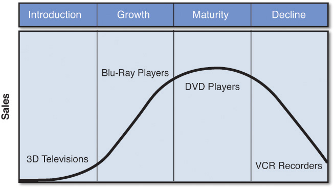
Introduction
During the introduction phase, there is very little history, if any, to go on, so forecasters tend to rely more on qualitative estimates that are generated both internally and externally. This information can come from sources such as market research; test markets, where that information can be extrapolated; similar items that you’ve sold before, which may or may not cannibalize other existing items; sales and customer estimates; advance orders to fill the distribution pipeline; and so forth.
Growth
As a product gains momentum through expanded marketing and distribution, some of the simpler time series methods may be used as minimal demand history becomes available.
A general rule of thumb in forecasting is that to generate a decent statistical forecast, you need at least 12 months of history. So, during this growth phase, forecasting is truly a blend of art and science, as both quantitative and qualitative methods are both used to create a blended forecast.
During the growth phase, it can be very easy to over- or underestimate forecasts, which can have dramatic effects on cost and service. So, great care must be taken, and all lines of communication must be established and open both internally and externally, to avoid surprises where possible (which in some cases, such as new distribution, may be hard to avoid).
Maturity
When a product reaches maturity, forecast accuracy tends to improve. For example, when I was in charge of forecasting at Church & Dwight for Arm & Hammer, it was relatively easy to forecast demand for a box of 1-pound baking soda because it had been around for more than 150 years. So, we could rely on simple models to forecast and didn’t need as much field information because the item wasn’t gaining many new customers. However, once a product reaches maturity, there are opportunities for brand extensions, which is what happened with baking soda. Baking soda actually has hundreds of applications; so, starting with refrigerator and freezer “packs,” baking soda gained new life (and new products). This went on to baking soda toothpaste, baking soda deodorant, and so on in the years that followed.
Decline
Once a product goes into its decline phase, besides sales having a general downward trend, the demand locations start to shift because the trend is not uniform. On top of that, other alternative channels not previously used such as dollar stores, discount chains, export, and so on may now be used.
Eventually, the product may be discontinued. However, forecasts must still be generated to run out existing inventory. Therefore, similar to the introductory phase, the forecaster relies more on qualitative than on quantitative methods.
Time Series Components
Time series models can contain some or all of the following components (see Figure 3.4).
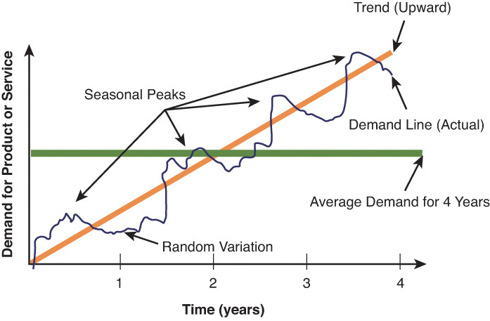
![]() Trend: An ongoing overall upward or downward pattern with changes due to population, technology, age, culture, and so on that is usually of several years or more in duration (for example, a fashion trend toward smaller bikinis).
Trend: An ongoing overall upward or downward pattern with changes due to population, technology, age, culture, and so on that is usually of several years or more in duration (for example, a fashion trend toward smaller bikinis).
![]() Cyclical: Repeating up and down movements typically affected by business cycle, political, and economic factors, which may vary in length and are usually 2 to 10 years in duration. There are often causal or associative relationships. Examples include economic recessions.
Cyclical: Repeating up and down movements typically affected by business cycle, political, and economic factors, which may vary in length and are usually 2 to 10 years in duration. There are often causal or associative relationships. Examples include economic recessions.
![]() Seasonal: A regular pattern of fluctuations due to factors such as weather, customs, and so on that occur within 1 year. Examples include natural occurrences such as climatic seasons or artificially created such as the school year or seller promotional plans.
Seasonal: A regular pattern of fluctuations due to factors such as weather, customs, and so on that occur within 1 year. Examples include natural occurrences such as climatic seasons or artificially created such as the school year or seller promotional plans.
![]() Random: Erratic fluctuations that are due to random variation or unplanned events such as union strikes and war, which are usually relatively short in nature and nonrepeatable.
Random: Erratic fluctuations that are due to random variation or unplanned events such as union strikes and war, which are usually relatively short in nature and nonrepeatable.
Because these components can be combined in different ways, it is usually assumed that they are multiplicative or additive.
Time Series Models
The most common quantitative time series models are as follows:
![]() Naive approach: Last period’s actual demand is used as this period’s forecast, without adjusting them or attempting to establish causal factors. (For example, if January sales were 100, then February forecasted sales will be 100.) It is simple, yet cost-effective and efficient.
Naive approach: Last period’s actual demand is used as this period’s forecast, without adjusting them or attempting to establish causal factors. (For example, if January sales were 100, then February forecasted sales will be 100.) It is simple, yet cost-effective and efficient.
![]() Moving average: The simple average of a demand over a defined number of time periods and is used if there is little or no trend because it tends to smooth historical data. Typically, more recent history is averaged to create the estimate. (For example, January–March sales are averaged to create an April forecast.)
Moving average: The simple average of a demand over a defined number of time periods and is used if there is little or no trend because it tends to smooth historical data. Typically, more recent history is averaged to create the estimate. (For example, January–March sales are averaged to create an April forecast.)
![]() Weighted moving average: An average that has multiplying factors to give different weights to data at different positions in the sample window. Typically used when some trend might be present because it treats older data as usually less important. The weights are based on experience and intuition and can be used to minimize the smoothing effect if desired.
Weighted moving average: An average that has multiplying factors to give different weights to data at different positions in the sample window. Typically used when some trend might be present because it treats older data as usually less important. The weights are based on experience and intuition and can be used to minimize the smoothing effect if desired.
For example:
Weighted moving average forecast for April = .6 * March sales + .3 * February sales + .1 * January sales
In this example, more weight has been given to March demand than to January and February to generate the April (and onward) forecast.
![]() Exponential smoothing: A smoothing technique used to reduce irregularities. It is a type of the weighted moving average model where weights decline exponentially, with the most recent observations given relatively more weight in forecasting than the older observations. Exponential smoothing requires an alpha smoothing constant (ranges between 0 and 1 and denoted by the symbol α), which is subjectively chosen.
Exponential smoothing: A smoothing technique used to reduce irregularities. It is a type of the weighted moving average model where weights decline exponentially, with the most recent observations given relatively more weight in forecasting than the older observations. Exponential smoothing requires an alpha smoothing constant (ranges between 0 and 1 and denoted by the symbol α), which is subjectively chosen.
For example:
New forecast = Last period’s forecast + .7 * (Last period’s actual demand – last period’s forecast)
In this example, the smoothing constant used of .7 will give a relatively high weighting or smoothing factor to an over- or undersell during the most recent month of history when generating the new forecast.
Associative Models
There are more sophisticated models known as associative models, such as linear regression (also known as least squares method) and multiple regression analysis, which use the relationship of an independent variable(s) (x) to predict a dependent variable (y). The reason it is called the least squares method is that the formula draws a best fit line through the historical data over time (that is, with the least deviation; see Figure 3.5). That formula can then be used to predict future values of y.
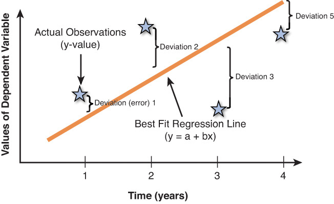
In linear regression, the relationship is defined as: y = a + bx, where a = the y axis intercept and b = the slope of the regression line.
A simple example of linear regression would be to derive and use this equation to predict future sales (y) by plugging in the sales budget (x) that we plan on using (with n being the total number of observations). If we know that the two variables are strongly correlated, we can easily derive the equation using historical sales personnel employment numbers along with historical sales.
To come up with this equation, we must solve for b and then a. The formula used to derive each are shown here:
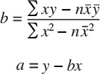
Once we have solved for a and b, we have our regression formula and can plug in future sales personnel employment estimates to predict future sales.
Correlation
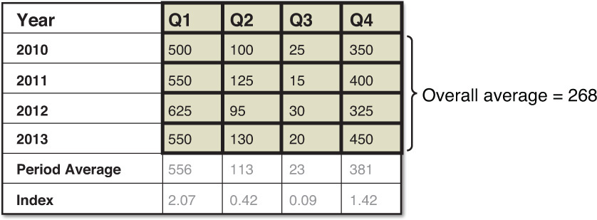
To measure correlation (that is, the mutual relation of two or more things), we calculate a correlation coefficient, also known as r, which is a measure of the strength and direction of the linear relationship between two variables that is defined as the (sample) covariance of the variables divided by the product of their (sample) standard deviations.
The range of correlation is 0 to 1. A perfect correlation between two variables would result in an r of +/–1. The lower the correlation between the two variables, the closer to 0 is the result.
Seasonality
In all the previously mentioned time series methods, as well as linear regression, we can apply what is known as a seasonality index. As mentioned, this may reflect actual seasonal sales of an item (that is, we sell more snow shovels in the winter) or can be artificially created (for example, a promotional calendar).
A seasonality index is relatively easy to create and can be applied to any of the previously discussed forecasting methods to give the forecast more realistic peaks and valleys.
To create a seasonality index, you must do the following:
1. Calculate an average for all item history (for all years and periods).
2. Average each period’s historical data.
3. Divide each period’s average by the overall average.
4. Apply the period index to the existing time series or linear regression forecast.
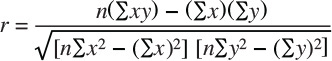
Suppose, for example, that a snow shovel that we sell has historical quarterly sales, as shown here.
We can create a seasonality index to apply to a flat moving average quarterly forecast of 100, for example. To do this, we first calculate an average for each period, and then calculate an overall average of 268. From there, we can calculate indices for each quarter by dividing their period averages by the overall average of 268.
If we had a quarterly forecast for next year of 100/quarter, we could apply the seasonality index for each quarter to that forecast. The resulting quarterly forecasts would be: Q1 = 2.07 * 100, or 207 shovels; Q2 = .42 * 100, or 42 shovels; Q3 = .09 * 100, or 9 shovels; and Q4 = 1.42 * 100, or 142 shovels.
As mentioned previously, seasonality can be natural or induced. In either case, it can change over time and needs to be recalculated on an ongoing basis.
Multiple Regression
When more than one independent variable is going to be used to develop a forecast, linear regression can be extended to multiple regression, which allows for several independent variables. (For example, discounting, promotions, advertising, and so on may all have an impact on sales to one degree or another.) The formula for this is: y = a + b1 x1 + b2 x2 ... (similar to the least squares formula, except with multiple independent variables). This is quite complex and generally done with the help of statistical software.
In the end, you will want to arrive at the best combination of independent variables for the best possible forecast. A statistic called an r-squared or coefficient of determination, which is the square of the correlation coefficient mentioned earlier and is a measure of the strength of the correlation between y and the various combination of x’s, is calculated. The closer to 1.0 the r-squared is, the better the correlation, and hopefully, the more accurate the forecast.
There are many other statistical methods used, ranging from simple to very complex. The best-in-class methods of forecasting use a blend of qualitative and quantitative methods that include collaboration both internally with staff from various departments, including sales, marketing, and finance, and externally with customers and suppliers.
Forecasting Metrics
You cannot control and improve a process if you don’t measure it, so it is important to both establish targets and to then track and measure forecast accuracy. There are many ways to establish forecast targets, including historical data, contribution, and so on. The one I prefer is the ABC method, which is a way to classify items based on their sales velocity or contribution to profits and can be used to not only set forecasting targets but also in inventory planning and control, as discussed in the next chapter.
To under the ABC method, you needs to understand a phenomenon known as the Pareto principle or the 80/20 rule. It states that a relatively small number of your items generate a fairly large percentage of your sales or profits and are referred to as A items (for example, Whopper, fries, and Coke are A items at Burger King).
In forecasting, these A items require more time and effort put into them and typically have better accuracy as a result. The slower movers, known as B and C items, are somewhat less important and require less forecasting time and effort and typically have more variability (Myerson, 2014).
Forecast Error Measurement
Forecast accuracy is the difference between what was forecasted for a period and what was actually sold or shipped. It can be measured in whole units or as a percentage.
A number of methods are used to measure and monitor accuracy. The main ones are described in the following subsections.
Mean Absolute Deviation
Simply put, the mean absolute deviation (MAD) is a way to measure the overall forecast error in units over periods of time.
The actual calculation for the MAD is the sum of the absolute error in units divided by the number of occurrences and represented as follows:
Mean Squared Error
The mean squared error (MSE) is the average of the squared differences between the forecasted and actual values. Its formula is the sum of the square forecast errors divided by the number of occurrences and represented as follows:
Mean Absolute Percent Error
As opposed to the MAD and MSE, which can vary in size based on the volume sold of an item, the mean absolute percent error (MAPE) calculates the absolute percentage error. From my experience, this is the most common way for businesses to measure and control forecast accuracy.
Typically, targets are set by ABC code or other methods that highlight relative importance of items, with A type items generally having a smaller variance because they are major, everyday items and so more predictable. C items, because there are more of them with much smaller volume, tend to be more volatile and so tend to have greater forecast variance.
The MAPE is calculated as follows:
Tracking Signal
Over time, forecasts can tend to get out of control fast. As a result, it is a good idea to utilize what is known as a tracking signal.
The tracking signal is used to determine the larger deviation (in both plus and minus) of error in forecast, and is calculated by the following formula:
Usually, upper and lower control limits (UCL and LCL) for the number of MADs that the tracking signal represents. There are no “magic” numbers for the UCLs and LCLs, because they are somewhat subjective, but keep in mind that 1 MAD = .8 standard deviations.
In a normal distribution, 3 standard deviations (or +/–4 MADs), should include 99.9% of the occurrences. So, if your tracking signal starts exceeding those levels, it is a good indication that something isn’t right.
Demand Forecasting Technology and Best Practices
Computerized forecasting software has been around for a long time. It has evolved from the mainframe to the PC to the Web, from installed applications to cloud based on-demand software-as-a-service (SAAS). These systems range from simple spreadsheet calculations to sophisticated packaged software systems utilizing a variety of forecasting methods and are in some cases integrated with customers and suppliers for improved visibility and collaboration.
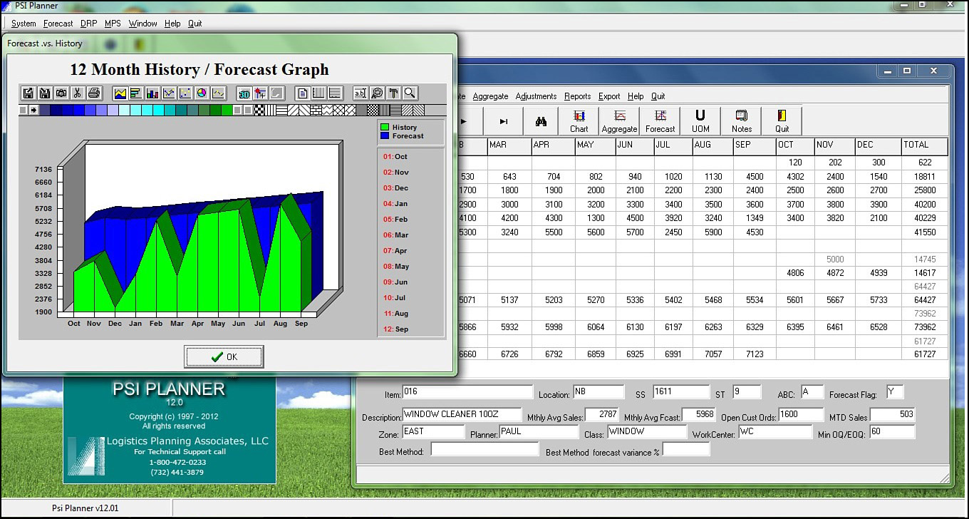
Historically, at least in terms of best-of-breed forecasting functionality, the software has been licensed from a separate vendor and integrated with the accounting or enterprise resource planning (ERP) software system. These integrated applications were then used to manage business and automate back-office functions for all facets of an operation, including product planning, development, finance, human resources, manufacturing processes, sales, and marketing. More recently, through development and acquisition, accounting and ERP vendors are increasingly adding this and other nontraditional functionality to their systems (see Figure 3.6).
Yet, with all of this, according to a KPMG advisory global survey of 544 senior executives (KPMG, 2007), nearly all organizations still use spreadsheets for some parts of the process; more worryingly, 40 percent of them rely solely on spreadsheets to produce the forecast. As a result, this leaves major chances for losses in efficiency and for redundancies in work processes.
However, the KPMG advisory found that the following separated the best in class from the rest regarding forecasting:
![]() Tend to take forecasting more seriously as they hold managers accountable for agreed-upon forecasts, incentivize managers for forecast accuracy, and use the forecast for ongoing performance management
Tend to take forecasting more seriously as they hold managers accountable for agreed-upon forecasts, incentivize managers for forecast accuracy, and use the forecast for ongoing performance management
![]() Look to enhance quality beyond the basics by incorporating scenario planning and use external market reports and data more often
Look to enhance quality beyond the basics by incorporating scenario planning and use external market reports and data more often
![]() Work harder at it by updating and reviewing forecasts more often and more formally and tend to use packaged forecasting software systems more often rather than just spreadsheets
Work harder at it by updating and reviewing forecasts more often and more formally and tend to use packaged forecasting software systems more often rather than just spreadsheets
Now that we have answered the demand question, the next step in most goods-oriented planning processes is this: How much and when do we need to produce or purchase product?