
5. Aggregate Planning and Scheduling
After we’ve made our best estimate of a demand forecast for goods or services and netted it against our current and targeted inventory position to determine our future inventory requirements, it becomes necessary to make sure that we have enough capacity to meet the anticipated demand.
When we think of planning the capacity for a goods or service business, we typically think in terms of three time horizons:
![]() Long range (1–3+ years): Where we need to add facilities and equipment that have a long lead time.
Long range (1–3+ years): Where we need to add facilities and equipment that have a long lead time.
![]() Medium range (roughly 2 to 12 months): We can add equipment, personnel, and shifts; we can subcontract production and/or we can build or use inventory. This is known as aggregate planning.
Medium range (roughly 2 to 12 months): We can add equipment, personnel, and shifts; we can subcontract production and/or we can build or use inventory. This is known as aggregate planning.
![]() Short range (up to 2–3 months): Mainly focused on scheduling production and people, as well as allocating machinery, generally referred to as production planning. It is hard to adjust capacity in the short run because we are usually constrained by existing capacity.
Short range (up to 2–3 months): Mainly focused on scheduling production and people, as well as allocating machinery, generally referred to as production planning. It is hard to adjust capacity in the short run because we are usually constrained by existing capacity.
The supply chain and logistics function must actively support all of these ranges by supplying material and components for production and product to the customer, and in fact, it has many of its own capacity constraints in terms of its distribution and transportation services.
In many service organizations, the actual work of capacity and supply planning for the production of inventory may be partially or totally in another organization, as is the case of retailers or wholesalers. But even in those instances, retail and wholesale supply chain organizations are intertwined with the vendor’s manufacturing process. So, they should participate, support, and integrate vendor production plans into their own processes when possible. In addition, service organizations have capacity constraints in terms of various resources that are impacted by inventory levels (labor, warehouse capacity, back room retail storage, shelf space, and so on). Therefore, it is well worth understanding the aggregate planning process no matter where you are in the supply chain.
The Process Decision
Stepping back for the moment, it should be understood that all organizations, both goods and services, have to make what is known as the process decision—that is, how the goods or services are to be delivered.
In most established organizations, there is already an existing process that is usually based on the industry’s and management’s competitive strategy.
Goods and Service Processes
Process choices in goods and service industries can be defined and delineated by what has become to be known as the product-process matrix (Hayes & Wheelwright, 1979; see Figure 5.1). In this model, an organization’s process choices are based on both the volume produced and variety of products. At the upper left of the chart, companies are considered process oriented or focused, and those in the lower right are considered product focused. The ultimate decision of where a firm locates on the matrix is determined by whether the production system is organized by grouping resources around the process or the product.
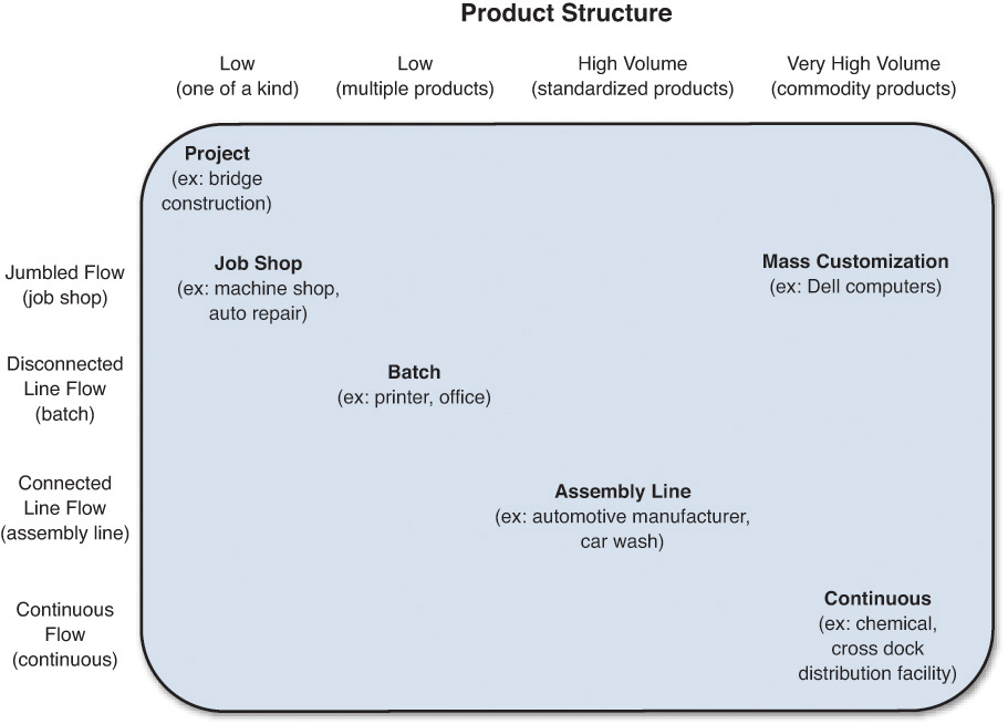
Project Process
Some industries, such as construction or pharmaceutical, are for the most part project oriented. where they typically make one-off types of products. They are usually customer specific and too large to be moved; so people, equipment, and supplies are moved to where they are being constructed or worked on.
Job Shop Process
Job shops typically make low-volume, customer-specific products. Machine shops, tool and die manufacturers, and opticians (that is, prescription glasses) are primary examples of a job shop. As such, they require a relatively high level of skill and experience because they must create products based on the customer’s design and specifications.
Each unique job travels from one functional area to another, usually with its own piece of equipment, according to its own unique routing, requiring different operations, different inputs, and requiring varying amounts of time.
Job shops can be extremely difficult to schedule efficiently.
Batch Process
Companies that run a batch process deliver similar items and services on a repeat basis, usually in larger volumes than a job shop. Batch processes have average to moderate volumes, but variety is still too high to justify dedicating many resources to an individual product or service. The flow tends to have no standard sequence of operations throughout the facility. They do tend to have more substantial paths than at a job shop, and some segments of the process may have a linear flow.
Examples of batching processes include scheduling air travel, manufacturing apparel or furniture, producing components that supply an assembly line, processing mortgage loans, and manufacturing heavy equipment.
Assembly Line or Repetitive Process
When product demand is high enough, an assembly line or repetitive process, also referred to as mass production, may be used. Assembly line processes tend to be heavily automated, utilizing special-purpose equipment, with workers usually performing the same operations for a production run in a standard flow. In many cases, a conveyor type system links the various pieces of equipment used.
Examples of this include automotive manufacturing (the classic example) and assembly lines. In service industries, examples include car washes, registration in universities, and fast-food operations.
Continuous Flow Process
A continuous flow process, as the name implies, flows continuously rather than being divided into individual steps. Material is passed through successive operations (that is, refining or processing) and eventually come out the end as one or more products. This process is used to produce standardized outputs in large volumes. It usually entails a limited and standardized product range and is often used to manufacture commodities. Very expensive and complex equipment is used, so these facilities tend to produce in large quantities to gain economies of scale to spread the considerable fixed costs over as much volume as possible so that the cost per individual pound or unit is as low as possible. Labor requirements are on the low side and typically involve mainly monitoring and maintaining of equipment.
Examples of this include chemical, petroleum, and beverage industries. This type of process is less common in service industries, but a good emerging example in supply chain are cross-dock distribution facilities, which move finished goods product through a distribution facility in as little as 24 to 48 hours.
Mass Customization
Mass customization is a process that produces in high volume and delivers customer-specific product in small batches and can provide a business with a competitive advantage and maximum value to the customer. It is a relatively new frontier for most goods and service businesses, and as a result, there aren’t that many examples of it.
In manufacturing, Dell computer is a primary example used by many because they allow customers to more or less assemble their own personal computers (PCs) online. Dell then assembles, tests, and ships the PCs directly to the customer in as little as 24 to 48 hours. Some clothing companies manufacture blue jeans to fit an individual customer.
In service industries such as financial planning and fitness, the service is customized specifically to meet the individual needs and therefore is an example of mass customization.
Planning and Scheduling Process Overview
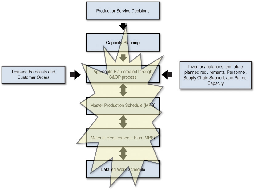
An aggregate plan, also known as a sales & operations plan (S&OP), is a statement of a company’s production rates, workforce, and inventory levels based on estimates of customer requirements and capacity limitations (see Figure 5.2).
Many service organizations perform aggregate planning in the same way as goods organizations, except that there is more of a focus on labor costs and staffing because it is critical to the service industry (and pure service companies don’t have inventory to manage, other than supplies).
A variety of methods can be used for aggregate planning, from simple spreadsheets to packaged software using algorithms such as the transportation method of linear programming, which is an optimization tool to minimize costs.
Graphical tools can also be used to supplement this process to allow the planner to compare different approaches to meeting demand (see the discussion about supply options later in this chapter).
As the name implies, the plan is usually stated in terms of an aggregate, such as product family or class of products, and displayed in monthly or quarterly time periods. It will determine resource capacity to meet demand in the short to medium term (3 to 12 months) and is usually accomplished by adjusting capacity (that is, supply) or managing demand.
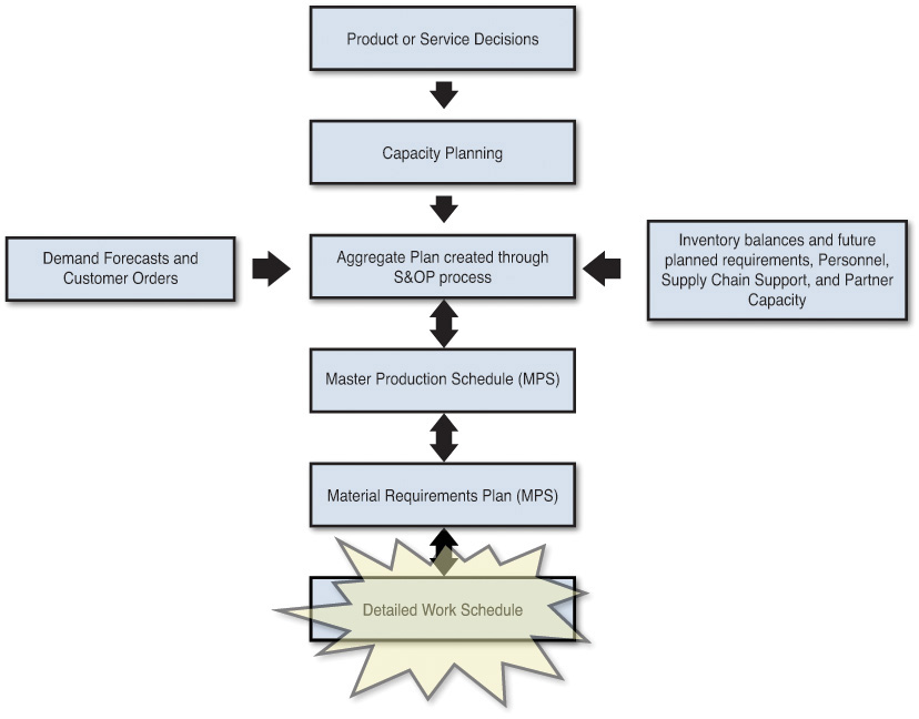
Once the aggregate plan is formalized, it is then disaggregated to create a master production schedule (MPS) for independent demand inventory (that is, finished goods), which is also referred to by many as a production plan. The MPS is stated in stock keeping unit (SKU) production requirements, usually in daily, weekly, or sometimes monthly time periods.
The MPS is then exploded using a bill of materials (BOM), which is basically a recipe of ingredients (that is, dependent demand) that goes into the final product (that is, independent demand). This activity is known as material requirements planning (MRP).
Once MRP has been run and material availability confirmed, a short-term or detailed work schedule is created. This schedule is where the rubber meets the road because this is a schedule of the actual work to be done, resulting in either meeting or not meeting customer requirements. The work schedule is usually in days or even hours and goes out up to a week or so. It has the specifics as to what product or service will be delivered, when, and who will deliver it.
Aggregate Planning
Aggregate planning, also referred to as sales & operations planning (S&OP), is an operational activity that generates an aggregate plan (that is, for product or service families or classes) for the production process for a period of 2 to 18 months. The idea is to ensure that supply meets demand over that period and to give an idea to management as to material and other resource requirements required and when, while keeping the total cost of operations of the organization to a minimum.
S&OP Process
Best practice companies have a structured S&OP process to ensure success for aggregate/S&OP planning. The executive S&OP process itself (see Figure 5.3) actually sits on top of the number crunching and analysis being done at a lower level of the organization and involves a series of meetings prior to a final S&OP executive-level meeting, which are used to create, validate, and adjust detail demand and supply plans. The meetings are as follows:
![]() Demand planning cross-functional meeting (Step 2): Generated forecasts are reviewed with a team that may include representatives from supply chain, operations, sales, marketing, and finance. As mentioned in Chapter 3, “Demand Planning,” forecasts have been generated statistically and aggregated in a format that everyone can understand and confirm. (For example, sales might want to see forecasts and history by customer in sales dollars.)
Demand planning cross-functional meeting (Step 2): Generated forecasts are reviewed with a team that may include representatives from supply chain, operations, sales, marketing, and finance. As mentioned in Chapter 3, “Demand Planning,” forecasts have been generated statistically and aggregated in a format that everyone can understand and confirm. (For example, sales might want to see forecasts and history by customer in sales dollars.)
![]() Supply planning cross-functional meeting (Step 3): After confirmed forecasts have been netted against current on-hand inventory levels to create production/purchasing plans. Again, this data will usually be reviewed in the aggregate by product family in units, for example.
Supply planning cross-functional meeting (Step 3): After confirmed forecasts have been netted against current on-hand inventory levels to create production/purchasing plans. Again, this data will usually be reviewed in the aggregate by product family in units, for example.
![]() Pre-S&OP meeting (Step 4): Data from the first demand and supply meetings are reviewed by department heads to ensure that consensus has been reached.
Pre-S&OP meeting (Step 4): Data from the first demand and supply meetings are reviewed by department heads to ensure that consensus has been reached.
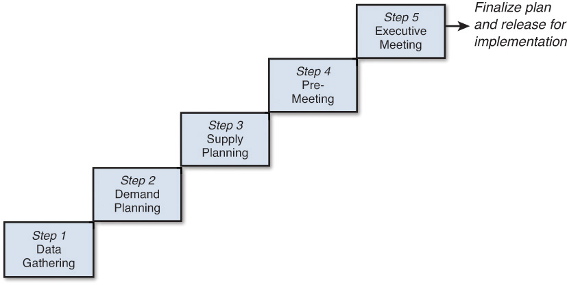
The discussions from this series of monthly management meetings highlight issues and look at possible resolutions before the outcome of the discussions is presented to the senior management team as a series of issues to be resolved. These issues form the basis of the executive S&OP meeting (Step 5).
The actual aggregate plan requires inputs such as the following:
![]() Resources and facilities available to the organization.
Resources and facilities available to the organization.
![]() Demand forecast with appropriate time horizon and planning buckets.
Demand forecast with appropriate time horizon and planning buckets.
![]() Cost of various alternatives and resources. This includes inventory holding cost, ordering cost, and cost of production through various production alternatives such as subcontracting, backordering, and overtime.
Cost of various alternatives and resources. This includes inventory holding cost, ordering cost, and cost of production through various production alternatives such as subcontracting, backordering, and overtime.
![]() Organizational policies regarding the usage of these alternatives.
Organizational policies regarding the usage of these alternatives.
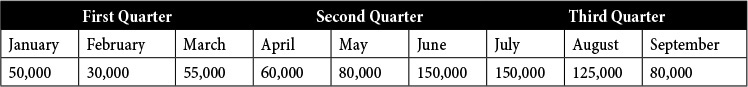
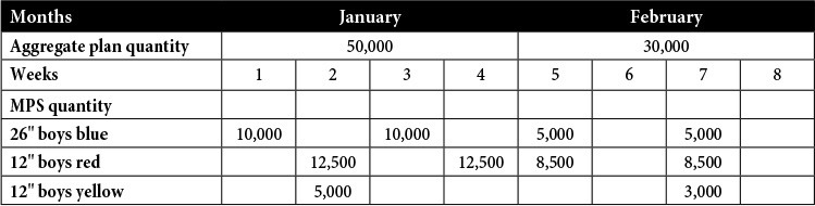
Table 5.1 is an example of an aggregate plan for a company that manufactures bicycles.
Some companies start with an aggregate plan and disaggregate to an MPS (that is, SKU level), and others start at the MPS and then aggregate to a class or family of products or services. In any case, the plans, at all levels, including detailed work schedule, are tested for various constraints (manpower, machine, and material) and then adjusted accordingly.
Integrated Business Planning
Note that there is a movement or evolution toward what has been called integrated business planning (IBP) or advanced S&OP for some leading organizations, which moves from fundamental demand and supply balancing to a broader, more integrated strategic deployment and management process.
On the operations side, manufacturing develops plans to balance demand and supply but do not always know whether the plan will meet the budgets on which the company’s revenue and profit goals are based. The sales department may agree to quotas that meet finance’s revenue goals without a detailed understanding of what manufacturing can deliver. IBF attempts to bridge those gaps by making sure that revenue goals and budgets are validated against a bottom-up operating plan, and that the operating plan is reconciled against financial goals.
S&OP in Retail
Also, although S&OP has been a best practice in manufacturing for 25 or so years, the retail industry has been slow to adapt it to their planning processes. The migration toward a broader IBF mentioned earlier for manufacturing may prove to be an impetus to pull retailers into using an S&OP process. In any case, when it is used in retail, the S&OP process is similar to that used by manufacturers. The main differences are that the sponsors and titles of each step as well as the details of each review such as issues, data, and decisions are different.
Demand and Supply Options
During the aggregate planning process, when trying to match supply with demand at the lower cost and highest service, an organization has options to adjust both demand and supply capacity.
Demand Options
These options refer to the ability to adjust customer demand to fit that demand to current available capacity. These options include the following:
![]() Influence demand: This can be accomplished to some degree via advertising, pricing, promotions, and price cuts. Examples including using early-bird meals in a restaurant or discounts offered if you buy before a certain date. These methods might not always have enough of an effect on demand to free up capacity.
Influence demand: This can be accomplished to some degree via advertising, pricing, promotions, and price cuts. Examples including using early-bird meals in a restaurant or discounts offered if you buy before a certain date. These methods might not always have enough of an effect on demand to free up capacity.
Also, as discussed previously, the use of heavy promotions and discounting can also have the negative bullwhip effect as a consequence (thus the reason that some companies have gone to everyday low pricing).
![]() Backorders: These occurs when a goods or service organization gets orders that they cannot fulfill. In many cases, customers are willing to wait. In others, it can result in lost sales. In some industries such as grocery stores, backorders are not used. Instead, if an item is out of stock, it is cut from the order and reordered next time. This is, of course, dangerous if your product is substitutable, because it might not be reordered next time.
Backorders: These occurs when a goods or service organization gets orders that they cannot fulfill. In many cases, customers are willing to wait. In others, it can result in lost sales. In some industries such as grocery stores, backorders are not used. Instead, if an item is out of stock, it is cut from the order and reordered next time. This is, of course, dangerous if your product is substitutable, because it might not be reordered next time.
![]() New or counter seasonal demand: This can be used to balance demand by season. For example, a company that sells lawn mowers may begin production of snow blowers. Companies must be careful to not go beyond their expertise or base markets.
New or counter seasonal demand: This can be used to balance demand by season. For example, a company that sells lawn mowers may begin production of snow blowers. Companies must be careful to not go beyond their expertise or base markets.
Supply Capacity Options
These options refer to the ability of an organization to adjust its available resource capacity to meet demand and include the following:
![]() Hire and lay off employees: As demand hits peaks and valleys, flexibility in the workforce can be used to compensate for these fluctuations. Although this can prove beneficial to the company, it can also have risks and costs in terms of unemployment and new-hire training costs.
Hire and lay off employees: As demand hits peaks and valleys, flexibility in the workforce can be used to compensate for these fluctuations. Although this can prove beneficial to the company, it can also have risks and costs in terms of unemployment and new-hire training costs.
![]() Overtime/idle time: Most companies have the ability to run some overtime when things get busy. The opposite may be true when things slow down, by moving idle workers to other jobs, at least to some extent. Equipment and workers efforts, to some degree, can also be sped up or slowed down. Although this might extend capacity a bit in the short term, employees may burn out. In the case of slack demand, profitability may suffer as a result of having too many workers doing make work.
Overtime/idle time: Most companies have the ability to run some overtime when things get busy. The opposite may be true when things slow down, by moving idle workers to other jobs, at least to some extent. Equipment and workers efforts, to some degree, can also be sped up or slowed down. Although this might extend capacity a bit in the short term, employees may burn out. In the case of slack demand, profitability may suffer as a result of having too many workers doing make work.
![]() Part-time or temporary workers: This is especially common for contract manufacturers and in the service industry during the holiday season. It isn’t usually an option in more technical jobs, other than some exceptions such computer programming and nursing. Also, quality and productivity may suffer as a result of this approach.
Part-time or temporary workers: This is especially common for contract manufacturers and in the service industry during the holiday season. It isn’t usually an option in more technical jobs, other than some exceptions such computer programming and nursing. Also, quality and productivity may suffer as a result of this approach.
![]() Subcontracting (or contract manufacturing): Very common in some industries, such as cosmetics and household and personal-care products, especially when the demand for a new item is uncertain or a company doesn’t yet have the capability to make the product. The downside is that costs may be greater because the subcontractor has to make a profit too, quality may suffer a bit because you have less control, and the fact you may be working with a future competitor.
Subcontracting (or contract manufacturing): Very common in some industries, such as cosmetics and household and personal-care products, especially when the demand for a new item is uncertain or a company doesn’t yet have the capability to make the product. The downside is that costs may be greater because the subcontractor has to make a profit too, quality may suffer a bit because you have less control, and the fact you may be working with a future competitor.
![]() Vary inventory levels: Inventory may be produced before a peak season when excess capacity may be limited. However, it can also drive up holding costs, including obsolete or damaged inventory. An example of this is the ice cream industry, where ice cream can be produced in the winter and put in a deep freeze until the busy season starts.
Vary inventory levels: Inventory may be produced before a peak season when excess capacity may be limited. However, it can also drive up holding costs, including obsolete or damaged inventory. An example of this is the ice cream industry, where ice cream can be produced in the winter and put in a deep freeze until the busy season starts.
Aggregate Planning Strategies
Three general aggregate planning strategies are commonly used, and use many of the demand and supply options discussed earlier:
![]() Level plans: Use a constant workforce and produce similar quantities each time period. This method uses inventories and backorders to absorb demand peaks and valleys and therefore tends to increase inventory holding costs.
Level plans: Use a constant workforce and produce similar quantities each time period. This method uses inventories and backorders to absorb demand peaks and valleys and therefore tends to increase inventory holding costs.
![]() Chase plans: This method minimizes finished goods inventories by adjusting production and staffing to keep pace with demand fluctuations. It looks to match demand by varying either workforce level or output rate. This can, of course, negatively affect productivity and costs.
Chase plans: This method minimizes finished goods inventories by adjusting production and staffing to keep pace with demand fluctuations. It looks to match demand by varying either workforce level or output rate. This can, of course, negatively affect productivity and costs.
![]() Mixed strategies: Probably used the most with a mix of both of the first two methods. In some cases, inventory is increased ahead of rising demand, and in other cases, backorders are used to level output during extreme peak periods. There may be layoff or furlough of workers during the slower, extended periods, and companies may subcontract production or hire temporary workers to cover short-term peak periods. As an alternative to layoffs, workers may be reassigned to other jobs, such as preventive maintenance, during slow periods.
Mixed strategies: Probably used the most with a mix of both of the first two methods. In some cases, inventory is increased ahead of rising demand, and in other cases, backorders are used to level output during extreme peak periods. There may be layoff or furlough of workers during the slower, extended periods, and companies may subcontract production or hire temporary workers to cover short-term peak periods. As an alternative to layoffs, workers may be reassigned to other jobs, such as preventive maintenance, during slow periods.
An example of this is where a company has two production facilities that manufacture the same products, one on the East Coast and one on the West Coast. If one plant has a distinct cost advantage, it may make sense to sometimes shift production to the lower-cost plant and expand its service area temporarily, such as during a slow period of demand. This will, of course, result in less production required at the lower-cost plant during those periods, possibly requiring layoffs. This decision is not to be taken lightly and must consider the total landed cost of the product for each plant, including transportation and distribution to the customer.
Master Production Schedule
Once the S&OP process has been completed, the aggregate plan is disaggregated into a master production schedule (MPS), which shows net production requirements for the next 2 to 3 months, usually in weekly or monthly time periods by SKU for independent demand items (see Table 5.1). This is known as time phased planning.
The net requirements above and beyond existing known ones, which are referred to as scheduled receipts, are called planned orders and planned receipts, the only difference being that planned orders are planned receipts that have been offset by the item’s lead time.
Note that the lead time for manufacturing, which is the time required to manufacture an item, is the estimated sum of order preparation time, queue time, setup time, run time, move time, inspection time, and putaway time. In the case of purchased items, the lead time is usually stated by the vendor and may or may not include inbound transit times.
Production Strategies
Manufacturers usually have one or a combination of the following production strategies:
![]() Make-to-stock (MTS): Production for finished goods is based on a forecast using predetermined inventory targets. Customer orders are then filled from existing stock, and those stocks are replenished through production orders. MTO enables customer orders to be filled immediately from available stock and allows the manufacturer to organize production in ways that minimize costly changeovers and other disruptions.
Make-to-stock (MTS): Production for finished goods is based on a forecast using predetermined inventory targets. Customer orders are then filled from existing stock, and those stocks are replenished through production orders. MTO enables customer orders to be filled immediately from available stock and allows the manufacturer to organize production in ways that minimize costly changeovers and other disruptions.
![]() Make-to-order (MTO): Produced specifically to customer order. Usually standardized (but low volume) or custom items produced to meet the customer’s specific needs. MTO environments are slower to fulfill demand than MTS and assemble-to-order environments (described next) because time is required to make the products from scratch. There also is less risk involved with building a product when a firm customer order is in hand.
Make-to-order (MTO): Produced specifically to customer order. Usually standardized (but low volume) or custom items produced to meet the customer’s specific needs. MTO environments are slower to fulfill demand than MTS and assemble-to-order environments (described next) because time is required to make the products from scratch. There also is less risk involved with building a product when a firm customer order is in hand.
![]() Assemble-to-order (ATO): Products are assembled from components after the receipt of a customer order. The customer order initiates assembly of the customized product. This strategy can prove useful when there are a large number of end products, based on the selection of options and accessories that can be assembled from common components. (This is one example of the concept of postponement.)
Assemble-to-order (ATO): Products are assembled from components after the receipt of a customer order. The customer order initiates assembly of the customized product. This strategy can prove useful when there are a large number of end products, based on the selection of options and accessories that can be assembled from common components. (This is one example of the concept of postponement.)
![]() Engineer-to-order (ETO): This strategy uses customer specifications that require unique engineering design, significant customization, or new purchased materials. Each customer order results in a unique set of part numbers, bills of material (that is, items required to make the product), and routings (that is, steps to manufacture a product).
Engineer-to-order (ETO): This strategy uses customer specifications that require unique engineering design, significant customization, or new purchased materials. Each customer order results in a unique set of part numbers, bills of material (that is, items required to make the product), and routings (that is, steps to manufacture a product).
For the service industry, the MPS may only be an appointment book or log to make sure that capacity (in this case, skilled labor or professional service) is in balance with anticipated demand.
Depending on the production strategy used, the production requirements in the MPS can be expressed based on a forecast, customer orders, or modules that are required for the manufacture of other items (for example, Table 5.2).
System Nervousness
Frequent changes to the MPS (or subsequently, the material requirements plan, as discussed shortly) can cause what is known as system nervousness, where small changes, usually as a result of updating the MPS plan too often, causes major changes to the requirements plan.
To avoid this, many companies use a time fence, whereby the planning horizon is broken into two parts:
![]() Demand (or firm) time fence (DTF): A designated period where the MPS is frozen (that is, not changes to current schedule). The DTF starts with the present period, extending as several weeks into the future. It can only be altered by senior management. Unfortunately all too often from what I’ve seen, the frozen segment is changed often due to firefighting and customer emergencies.
Demand (or firm) time fence (DTF): A designated period where the MPS is frozen (that is, not changes to current schedule). The DTF starts with the present period, extending as several weeks into the future. It can only be altered by senior management. Unfortunately all too often from what I’ve seen, the frozen segment is changed often due to firefighting and customer emergencies.
![]() Planning time fence (PTF): A designated period during which the master scheduler is allowed to make changes. The PTF starts after the DTF ends and extends several weeks or more into the future.
Planning time fence (PTF): A designated period during which the master scheduler is allowed to make changes. The PTF starts after the DTF ends and extends several weeks or more into the future.
Material Requirements Planning
After the MPS has been solidified, it can then be exploded through a bill of materials (BOM) file to determine raw material and component (that is, dependent demand) requirements.
The information needed to run a Material Requirements Planning (MRP) model includes the MPS, a BOM, inventory balances, lead times, and scheduled receipts (that is, purchase orders and production work orders). All of these inputs need to be accurate and up to date. Otherwise, it’s the old garbage in, garbage out situation, resulting in poor execution and ultimately customer dissatisfaction.
All the inputs are fairly straightforward, but it would be helpful at this point to delve a little bit into the BOM.
Bill of Materials
A BOM is like a recipe for a product. (In fact, in the case of food, it is.) A BOM file has a defined structure to it. In this structure, the independent demand item is called the parent item (for example, 26-inch boys blue bike) and any dependent demand requirements (for example, two wheels for each bike) are called child items, with a quantity (2 / Bike in our example) of each child item needed to make each parent item. This is often referred to as the product structure (see Figure 5.4).
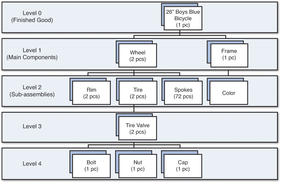
The finished good or parent item is referred to as being on level 0 and the child level 1. There can be multiple levels in a BOM, in which case the child item on level 1 of the wheel in the bike example can then be the parent to the child items of the rim, tire, spokes (that is, level 2), and so on.
MRP Mechanics
The calculations involved in an MRP system are fairly routine. Think of it as a giant calculator that crunches the information supplied to create net future replenishment requirements based on some user-defined parameters.
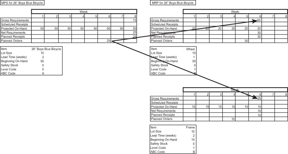
As mentioned previously, an MRP system is driven by the MPS (which may, in turn, potentially be driven by a DRP system). The mechanics of the MPS and MRP systems are basically the same, with the requirements from the MPS (independent demand) driving MRP requirements (dependent demand) via the BOM file.
In the bicycle example, Figure 5.5 illustrates the basic calculation where we have gross requirements (in MPS, gross is the forecast consumed by open customer orders) for the production of 75 bikes in week 8. Typically, safety stock or safety time targets would be in place for independent demand items, but for sake of simplicity, there is none in the example. Because we have 50 bikes in inventory, we need to produce an additional 25 units by week 8. To do so, we need to have 50 wheels and 25 frames available in week 6, after offsetting the components’ lead time, for the bike production. Through the BOM explosion, these requirements show up as gross requirements for the wheels and frames in MRP. The same netting calculations are then performed to create planned receipts and planned orders for the wheels and frames (and then level 2, level 3, and so on items).
Although it has been said that no safety stock or safety time are required for raw or components because it is factored into finished goods requirements, the reality is that quality and other issues may arise, as well as vendor minimum order quantities, which may call for safety stock as the prudent thing to do.
The actual quantity required is typically rounded up based on various lot-sizing techniques. They range from lot for lot (that is, exact requirements no matter how small), which is appropriate for just-in-time (JIT) operations, to economic order quantity (EOQ) calculations, and beyond.
For slow-moving items, an order time may be used, which basically states that the planned orders will be grouped together so that one larger order versus many frequent small orders will be placed. In the case of purchased material or parts, vendors may set order minimums (which can always be negotiated). Although this might result in greater holding costs, in the case of slower-moving items, it may be the right thing to do.
Note that in the case of both DRP and MRP, there are resource versions (versus requirement) that look beyond material requirements and consider other resources impacted such as labor, facilities, and equipment. Some are known as closed-loop systems, which allow for the planners to schedule work based on period capacity constraints using smoothing tools that allow the system (manually or automatically) to move requirements around to meet capacity based on priority rules set by the planner such as order splitting (running parts of a work order at two different times) and overlapping (part of a work order can move to a second operation while the rest is still on the first operation).
The planned orders for both independent and dependent demand are then used (either manually or sent electronically to either an enterprise resource planning [ERP] or accounting system) to create production work orders and purchase orders in what is known as short-term scheduling.
Short-Term Scheduling
As mentioned before, the short-term schedule (see Figure 5.6) is where the rubber meets the road, because effective schedules are necessary to meet promised customer delivery dates with the highest-quality product or service at the lowest possible cost.
Operations scheduling is the allocation of resources in the short term (down to days, hours, and even minutes in some cases) to accomplish specific tasks.
Scheduling includes the following:
![]() Assigning jobs to work centers/machines
Assigning jobs to work centers/machines
![]() Job start and completion times
Job start and completion times
![]() Allocation of manpower, material, and machine resources
Allocation of manpower, material, and machine resources
![]() Sequence of operations
Sequence of operations
![]() Feedback and control function to manage operations
Feedback and control function to manage operations
Scheduling techniques vary based on the facility layout and production process used.
Effective scheduling can support the supply chain to create a competitive advantage for an organization, as discussed earlier in this book.
Types of Scheduling
Two general types of operations scheduling help to determine the load or amount of work that is put through process centers:
![]() Forward scheduling: Plans tasks from the date resources become available to determine the shipping date or the due date and used in businesses such as restaurants and machine shops
Forward scheduling: Plans tasks from the date resources become available to determine the shipping date or the due date and used in businesses such as restaurants and machine shops
![]() Backward scheduling: Plans tasks from the due date or required-by date to determine the start date and/or any changes in capacity required and used heavily in manufacturing and surgical hospitals
Backward scheduling: Plans tasks from the due date or required-by date to determine the start date and/or any changes in capacity required and used heavily in manufacturing and surgical hospitals
In many cases, organizations may use a combination of both depending on the product or service.
The load put on a work center can be infinite (for example, unlimited capacity, such as in the basic MRP model) or finite (where capacity is considered).
Sequencing
Understanding and minimizing flow time is critical to good scheduling and the efficient utilization of resources. Flow time is the sum of 1) moving time between operations, 2) waiting time for machines or work orders, 3) process time (including setups), and 4) delays.
The concept of sequencing uses both priority rules to determine the order that jobs will be processed in and the actual job time, which includes both the setup and running of the job, to schedule efficiently.
Priority Rules
Although there are many priority rules, including the catchall emergency (that is, rush or priority customers), the basic rules are as follows:
![]() First come, first served (FCFS): Jobs run in the order they are received. Perhaps the fairest, although not always most efficient, way of scheduling.
First come, first served (FCFS): Jobs run in the order they are received. Perhaps the fairest, although not always most efficient, way of scheduling.
![]() Earliest due date (EDD): Work on the jobs due the soonest.
Earliest due date (EDD): Work on the jobs due the soonest.
![]() Shortest processing time (SPT): Shortest jobs run earlier to make sure that they are completed on time. Larger jobs will possibly be late as a result.
Shortest processing time (SPT): Shortest jobs run earlier to make sure that they are completed on time. Larger jobs will possibly be late as a result.
![]() Longest processing time (LPT): Start with the jobs that take the longest to get them done on time. This may work well for long jobs, but the others will suffer as a result.
Longest processing time (LPT): Start with the jobs that take the longest to get them done on time. This may work well for long jobs, but the others will suffer as a result.
![]() Critical ratio (CR): Jobs are processed according to smallest ratio of time remaining until due date to processing time remaining.
Critical ratio (CR): Jobs are processed according to smallest ratio of time remaining until due date to processing time remaining.
The planner can create schedules based on these methods (manually or automated) to both see the impact on job lateness and flow time and to determine what works best for the company and its customers. It might not always be possible to satisfy all customers, though.
Finite Capacity Scheduling
Finite capacity scheduling (FCS) is a short-term scheduling method that matches resource requirements to a finite supply of available resources to develop a realistic production plan. The MPS and MRP schedules are usually imported into this tool along with other information such as priority rules, setup times, and so on to create short-term daily and hourly schedules.
It uses not only rules-based methods, but also allows for the planner to make up to the minute changes and adjustments as well as perform what-if simulation analysis. They allow the planner to handle a variety of situations, including order, labor, and machine changes. The schedules in FCS are usually displayed in Gantt chart form (kind of a sideways bar chart, which can show planned as well as the current status of schedules) and can be accomplished using a range of tools from relatively simple spreadsheets to sophisticated optimization FCS software applications.
Service Scheduling
Although service industries need to schedule production and assembly of product (for example, restaurants), most are primarily interested in scheduling staff. To effectively schedule staffy, they use tools such as appointment systems (to control customer arrivals for service and consider patient scheduling), reservation systems (to estimate demand for service), and workforce scheduling systems (often using seniority and skill sets to manage capacity for service).
These can be manual or automated software systems depending on the size and complexity of the organization.
Technology
Similar to demand planning systems, supply planning tools range from simple spreadsheets (or even the back of an envelope) to sophisticated packaged software systems for optimization.
Much of the basic functionality discussed in this chapter, such as inventory control and management and MRP, is usually part of an organization’s ERP or accounting system. Other functions described, such as production and deployment planning and scheduling systems (for example, WMS, DRP, and FCS systems), are not, and may have to be licensed separately as add-ons and integrated with existing ERP and accounting systems.
Now that you have a good handle on the planning and scheduling processes and technologies for the supply chain, it’s time to take a look at supply chain management from both a strategic and operational viewpoint.