
Chapter 4. Green, Sustainable Materials
4.1. Introduction
Almost every engineering design involves the use of materials. If an engineering design is to be as sustainable as possible, the materials that are involved in the embodiment of the design should have light environmental and natural resource use footprints. Determining the magnitude of a material’s footprint is not straightforward, however. In this chapter, a three-pronged approach to characterizing the footprint of materials will be described.
To be used in an engineering design, a material must first be extracted and purified (refined), and the overall impact of this extraction and refining is the first component of the footprint. Once the material enters the production system, it can be reused and recycled, reducing the need for extraction processes. The extent to which various materials are reused and recycled, and the energy and other resources used in processing the materials, is a second component of the footprint. Finally, if a material is not reused or recycled but escapes into the environment, its environmental fate, persistence, human health impact, and ecological impact are a third component of the footprint. Methods for characterizing the environmental footprints associated with each of these steps (extraction, processing, and environmental release) are described in the next three sections. The chapter concludes by discussing methods for combining these assessments.
4.2. Environmental and Natural Resource Use Footprints of Material Extraction and Refining
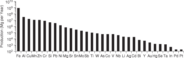
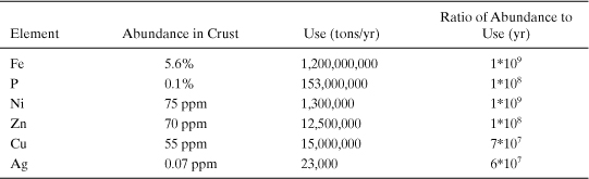
One of the simplest approaches for characterizing the footprints associated with the extraction and production of a material is to assess the material’s overall scarcity. Simply stated, if a material is scarce, it is likely to be energy-intensive to obtain and refine it, and the ability to meet large-scale demand will be limited. Elements vary widely in their natural abundance. Table 4-1 reports the relative abundance of materials in the Earth’s crust (note that this does not include oceans). The most common elements on a mass basis are, in descending order, O, Si, Al, Fe, Ca, Mg, and K. All of these elements are present at greater than 1% abundance in the Earth’s crust, and all are present in widely used commodity materials. In contrast, some widely used elements (Ag, Sn, Sb) are present at the ppm level or lower, on average, in the crust. Figure 4-1 shows the relative amounts of various elements that are produced each year for commercial applications (Gerst and Graedel, 2008).
Table 4-1. Abundance of Selected Elements in the Earth’s Crust (Mass Abundance)
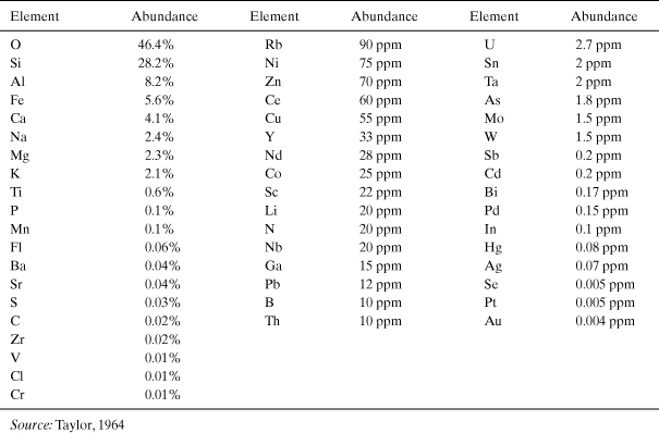
Figure 4-1. Annual production of elements for use in commerce (Reprinted with permission from Gerst and Graedel, 2008. Copyright 2008 American Chemical Society)
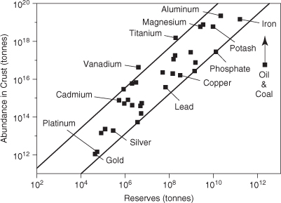
The extent to which elements are extracted can be quantitatively compared to the crustal abundance to produce one measure of the supply of the material. Example 4-1 examines the ratio of total crustal abundance to annual production rate. The result of the calculation in Example 4-1, the number of years at which current consumption rates could be sustained if all of the material in the Earth’s crust could be extracted, is a very simplistic measure of material supply. Not all of the elemental material in the Earth’s crust can be effectively extracted. Much of the material is simply present at concentrations that are too low to be extracted cost-effectively. Figure 4-2 shows the relationship between total crustal abundance and identified and economically extractable deposits (reserves). On average, only 1 in 107 to 109 tons of an element in the Earth’s crust is an economically viable reserve of the material. Example 4-2 examines the relationship between reserves and annual use rates for several commodity materials.
Figure 4-2. Relationship between total crustal abundance and reserves (Kesler, 1994)
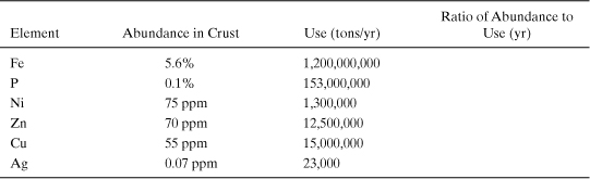
Example 4-1. Supplies and use of elements
Calculate the ratio of the abundance of materials in the Earth’s crust (tons) to the annual use of the materials (tons/yr). Assume an approximate mass for the crust of 2 * 1019 metric tons. This mass is based on a 40 km thickness for continental crust and a 3 km thickness for oceanic crust, with an average density of 3 g/cm3 (3 tons/m3).
Solution:
For example, for silver:
Abundance in crust * crustal mass/use rate = 7 * 10-8 * 2 * 1019 metric tons/ (2.3 * 104) = 6 * 107 yr
Example 4-2. Economically extractable supplies and use of materials
Calculate the ratio of the economically extractable materials in the Earth’s crust (reserves) to the annual use of the materials (tons/yr). The quantities of reserves identified in this exercise are derived from the U.S. Geological Survey (USGS, 2010).
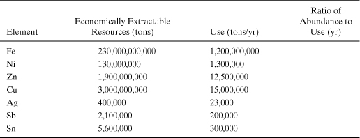
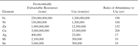
As illustrated in Example 4-1, the total amount of material available in the Earth’s crust is sufficient to support current rates of extraction indefinitely. However, Example 4-2 shows that the total amount of crustal material that is present in high enough concentrations to be economically recoverable is much lower than the total amount of material. This is because energy and other resources are required to purify materials into commercially useful forms. An approximate relationship between the concentration at which a material is found in a raw material and the cost to refine the material is shown in Figure 4-3. This concept—that the cost of a material is largely determined by the cost of extracting and purifying the raw material—is sometimes referred to as the Sherwood relationship, named after chemical engineering Professor T. Sherwood of MIT, who noted the relationship in the 1950s. Johnson et al. (2007) updated the data for the 21st century to create the information shown in Figure 4-3.
Figure 4-3. Metal prices (2004) as a function of dilution (1/concentration) of metals in commercial ores; the relationship illustrates the concept that the more dilute a material is in its native ore, the more expensive it will be to purify into a commodity material. (Reprinted with permission from Johnson et al., 2007. Copyright 2007 American Chemical Society)
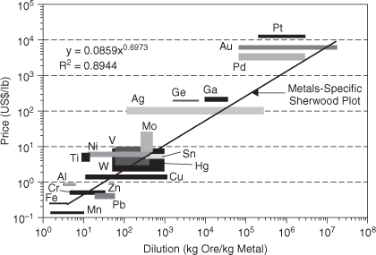
The relationship between prices and dilution in ores—the Sherwood relationship—is technology-dependent. As technologies continue to become more efficient, costs associated with material extraction can be reduced. There is, of course, a physical limit. A certain amount of entropy must be overcome to purify a material, and that imposes a minimum energy burden that must be overcome. As Example 4-3 shows, however, current technologies are far from those entropy limits.
Example 4-3. Energy burdens of material recovery (adapted from Allen, 1996)
To recover resources from raw materials, the minimum amount of energy that must be invested to concentrate the material is determined by the entropy that must be overcome in the purification.
a. To make an estimate of this energy, calculate the entropy of mixing that must be overcome in concentrating 1 kg of a metal present at 0.2 ppm (mole fraction basis) in water (imagine a process that seeks to harvest lithium from seawater to manufacture lithium-ion batteries). The entropy of mixing is given by
ΔS = –R Σ xi ln xi
where ΔS is the molar entropy of mixing, R is the gas constant, xi is the mole fraction of each component in the mixture, and the summation is done over all components in the mixture. Lithium has an atomic weight of 6.94.
b. The minimum energy required for separation (the energy required to overcome changes in entropy) is given by
ΔG = TΔS
where ΔG is the Gibbs free energy of mixing and T is the absolute temperature. Perform your calculation at room temperature and at 400K. Compare this minimum energy to a hypothetical process for recovering lithium. Assume that the lithium is obtained through a process that requires evaporating the seawater at near ambient pressure (boiling at near 400K). Calculate the energy required to heat the water from room temperature to 400K (assume that the heat capacity of water is 1 cal/g °K, 4.18 J/g °K, or 0.04 BTU/g °K) and to evaporate the water (assume that the heat of evaporation is 2270 J/g or 2.16 BTU/g).
c. If a gallon of fuel costs $3.00 and each gallon contains approximately 124,000 BTU, what are the energy costs to recover 1 kg of metal at room temperature and at 400K?
Solution:
a. Calculate the change in entropy per mole of mixture:
ΔS –R Σ xi ln xi = 2 cal/(°K mole) * 0.9999998 ln (0.9999998) + 0.0000002 ln(0.0000002) = -3 * 10-6 cal/(°K mole)
b. Noting that there are roughly 109/18 gram moles per million kilograms of solution (per 0.2 kg of metal), the change in entropy per kilogram of metal is 5*(109/18)* –3 * 10-6 cal/(°K mole) –833 cal/°K. At 300K the energy required to overcome this entropy change, per kilogram of lithium recovered, is 250 kcal; at 400K the energy required is 330 kcal.
c. At room temperature, the change in free energy is roughly 250 kcal per kilogram of metal. At 400K, the change is roughly 330 kcal per kilogram. Both quantities are negligible compared to the energy required to heat 5 million kg of water to 400K (1 cal/g °K * (400–300)°K * 5 * 109 g = 5 *1011 cal = 5 * 108 kcal). (Note that this does not include the heat of vaporization.)
d. The energy cost for heating 5 million kg of water to 400K is roughly $50,000 (5 * 1011 cal * 1 BTU/252 cal * $3/124,000 BTU = $48,000). While boiling seawater is not the only way to recover lithium, this simple example illustrates the difference between theoretical energy requirements and the actual energy requirements of material recovery systems.
The preceding examples demonstrate that the total amounts of resources available in the Earth’s crust are sufficient to supply commercial needs indefinitely. However, the amounts of various elements in the Earth’s crust that are present in high enough concentrations to be recoverable are limited. The primary limitations on recovering materials are economic. Energy and other resources are required to extract and purify materials, introducing costs. The costs are defined primarily not by physical laws (overcoming entropy) but by the technologies that are used, which continue to evolve.
The amounts of materials that can be economically recovered, referred to as reserves, are defined in multiple ways. Figure 4-4 summarizes these definitions. Reserves that are known and that have had their extent demonstrated, and that can be recovered at costs lower than current prices, are referred to as economically recoverable reserves. Demonstrated reserves that could be cost-effectively recovered, through either moderate improvements in technology or increases in price, are referred to as marginal reserves. Demonstrated reserves that are unlikely to be recoverable at any foreseeable price are referred to as subeconomic. Finally, demonstrated reserves can also lead to inferences that similar geological formations may contain similar reserves. These are referred to as inferred reserves, which can be economic, marginal, or subeconomic.
Figure 4-4. A reserve classification for minerals, the McElvey diagram (USGS, 2010, Appendix C)
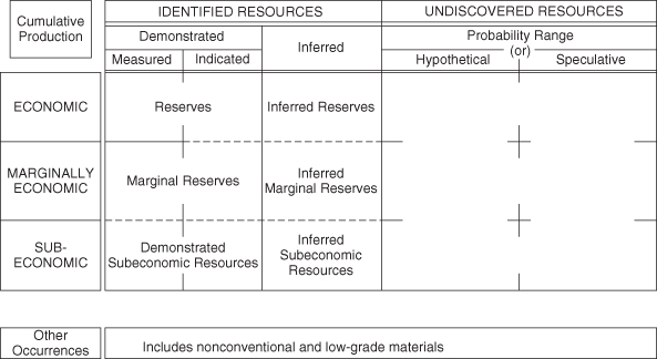
Demonstrated and inferred reserves may also be expanded as new areas are opened to exploration, so undiscovered reserves could expand all of the identified resources. Figure 4-4 shows the interrelationships between these ways of referring to reserves.
Example 4-4. McElvey diagram for gold
Using the mineral commodity summaries available from the U.S. Geological Survey (http://minerals.usgs.gov/minerals), identify the reserves for gold in the United States.
Solution: “An assessment of U.S. gold resources indicated 33,000 tons of gold in identified (15,000 tons) and undiscovered (18,000 tons) resources” (USGS, 2010).
Example 4-5. McElvey diagram for rare earth elements
Using the mineral commodity summaries available from the U.S. Geological Survey (http://minerals.usgs.gov/minerals), identify the U.S. production and global reserves for rare earth elements in the United States. If an average electric vehicle or plug-in hybrid electric vehicle requires 10 kg more rare earth elements than a conventional vehicle, by what percentage would rare earth metal use increase in the United States if 1 million of these vehicles were manufactured in the United States each year?
Solution: U.S. consumption of rare earth elements was roughly 5000 to 10,000 metric tons per year over the past five years. Almost all of this domestic use, and global use, comes from production in China. Undiscovered resources are believed to be extensive, resulting in an estimated total reserve of 99 million metric tons (USGS, 2010).
One million hybrid or electric vehicles would require roughly 10,000 metric tons (10 million kg) of rare earth elements, roughly doubling U.S. consumption.
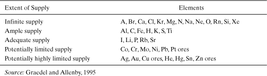
To summarize, the total amounts of resources available in the Earth’s crust are sufficient to supply commercial needs indefinitely. However, economic reserves are limited. Graedel and Allenby (1995) have evaluated the relative supplies of various elements and grouped them into the categories shown in Table 4-2. Multiple elements are grouped together in the table, since they are found in the same types of ores. For example, Cu ores typically also contain As, Se, and Te. Pt ores typically contain Ir, Os, Pa, Rh, and Ru. The element with the highest demand, or highest price, tends to drive the extraction of these ores. So, for example, mining of Zn produces Cd as a by-product, making it available at a price and a quantity that might not be possible if it were not associated with Zn.
Table 4-2. Supplies of the Elements
Overall, the key concept to take away from this analysis is that the total amount of materials in the crust is enormous. Since, in general, very little of this mass ever escapes the planet, the total amount of material is conserved and these materials will always be available. What does happen as resources are used, however, is that highly concentrated forms of various elements, extractable at low cost, are depleted. While the analyses presented in this section have focused on minerals and metals, the principles are generally valid.
As ever more dilute materials need to be extracted to satisfy demand, the energy and other resources required to perform that extraction, and consequently the cost of the material, increase. This suggests that a logical approach to the efficient use of materials would be to track the flows of materials. If materials, in concentrated form, can be recycled or reused, there is the potential to avoid additional extraction and to save energy. Tracking material flows in engineered systems is the topic of the next section.
4.3. Tracking Material Flows in Engineered Systems
Materials have a life cycle. They are extracted from the lithosphere or biosphere, processed into commodity materials, then products, then used and possibly reused, then eventually disposed of or leaked into the environment. The number of times that a material is reused or recycled before it is released into the environment can have a significant impact on its environmental footprint. In addition, different types of uses, for the same material, can lead to very different types of impacts.
Characterizing the flows and emissions of materials in manufacturing and use requires data on material and mineral flows entering the economy, and information on the wastes, emissions, and recycling structures. Data that enable this new generation of analyses are just emerging. Therefore, terminology and data analysis frameworks are still evolving. One set of terminology is shown in Figure 4-5.
Figure 4-5. Conceptual framework for analyzing material flows (National Research Council, 2003)
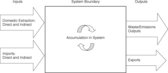
As shown in Figure 4-5, material flow analyses are performed on systems with well-defined boundaries. The system boundary might be the geopolitical boundaries of a nation, the natural boundaries of a river’s drainage basin, or the technological boundaries of a cluster of industries. The labels for the system inputs and outputs used in Figure 4-5 suggest that the system is a nation, but these inputs and outputs (domestic extraction, imports, and exports) could be labeled “feedstocks” and “products,” and the system would then appear to be a cluster of industries.
Figure 4-5 also identifies material inputs, material outputs, releases to the environment, and material accumulation as components of the material flow analysis. The system inputs and outputs are segregated into direct and indirect flows. Direct flows are those that are normally accounted for in engineering analyses, such as fuels, minerals, metals, and water. The indirect, or hidden, flows shown in Figure 4-5 are composed of materials such as mining overburdens and soil erosion from agricultural operations. These hidden material flows do not enter the economic system, yet they occur as a result of economic activity. Within the system, stocks are accumulated and materials are reused and recycled. As flows internal to the system are reengineered to incorporate more reuse and recycling, releases to air, water, and land can be reduced and demands for inputs are reduced.
Consider, as an example of material flow analyses, the element lead (Pb). Pb is a neurotoxin, and Pb exposure is associated with developmental delays (www.epa.gov/iris). Human exposure to Pb should therefore be minimized. Historically, some of the principal uses of lead have been as an octane enhancer in gasoline, in batteries, and in paint. The material flows of Pb in the United States in 1970 and in the mid-1990s are shown in Figure 4-6. As shown in the left-hand portion of the diagram, flows of Pb come from both extraction of geological resources (virgin materials) and recycled material. In 1970 the fraction of virgin material was 36% (450 tons recycled/1250 tons total usage), while in the mid-1990s the fraction had increased to 65% (910 tons recycled/1400 tons total usage). The Pb is incorporated into a variety of products; some products, when used as designed (such as lead paint applied outdoors or lead additives in gasoline), result in the release of Pb into the environment (dissipative uses). Other products, when used as designed (lead acid batteries), can be effectively recovered and recycled at the end of the product’s life (nondissipative uses).
Figure 4-6. Material cycles for lead in 1970 and the mid-1990s (USGS, 2000); flows are in thousands of metric tons per year
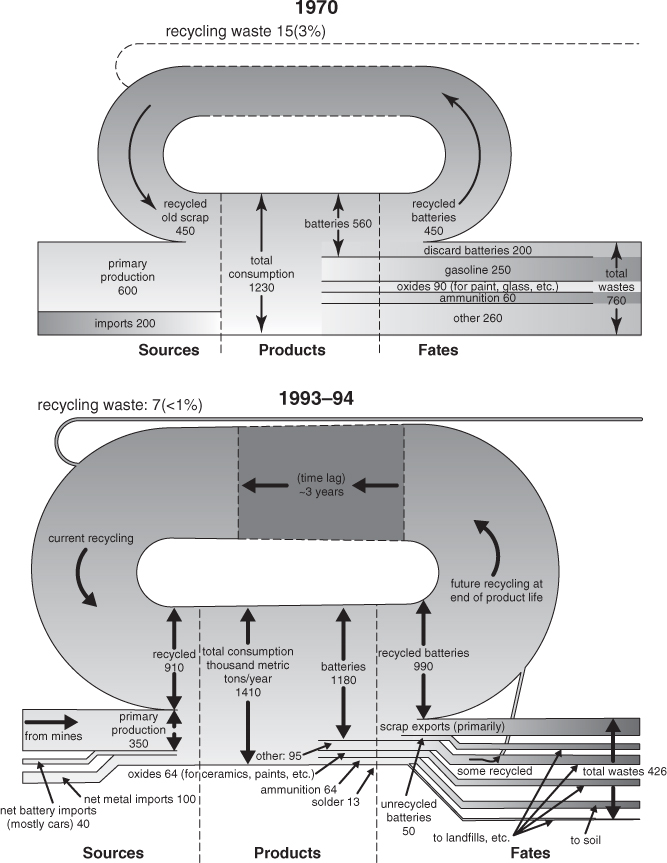
Figure 4-6 shows that the fraction of dissipative uses decreased significantly from 1970 until the mid-1990s in part because of the phaseout of many lead-based paints and lead additives in gasoline. Use of Pb in batteries increased significantly from 1970 through the mid-1990s, as the demand for starting-lighting-ignition batteries in vehicles increased.
Figure 4-6 can be expanded to incorporate additional types of flows, and Figure 4-7 illustrates some of those flows, using global use of iron as a case study. Figure 4-7 separates iron flows during production of products into production, fabrication/manufacturing, use, and waste management. There are flows between these stages of materials processing, for example, as “home” scrap within production operations is reprocessed. The material flow mapping of Figure 4-6 also shows flows of material from different processing stages into anthropogenic repositories (such as landfills) and the flows of material into durable goods (stock). Overall, however, the mapping provides much of the same information as was illustrated in Figure 4-6. Flows of crude ore from the lithosphere (virgin ore) can be compared to various types of recycling; losses to the environment can be compared to total use and stocks.
Figure 4-7. Global flows of iron in 2000 (Wang et al., 2007; reprinted with permission, STAF Project, Yale University)
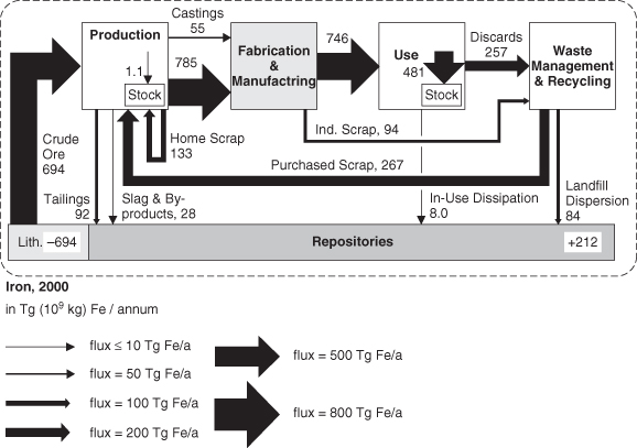
Example 4-6. Global material balance for iron
Material flow information, of the type shown in Figure 4-7, typically comes from multiple sources, and material balances can be used to assess the consistency of the information. At the most macroscopic level, the basic material balance equation, in = out + accumulation, can be translated into crude ore in = flows to repositories = stock accumulation. Determine whether the flows in Figure 4-7 satisfy a material balance.
Solution:
crude ore in = flows to repositories + stock accumulation crude ore in = 694 Tg/annum
Flows into repositories + stock accumulation = 212 + 481 = 693 Tg/annum
So, within rounding error, the flows satisfy a material balance.
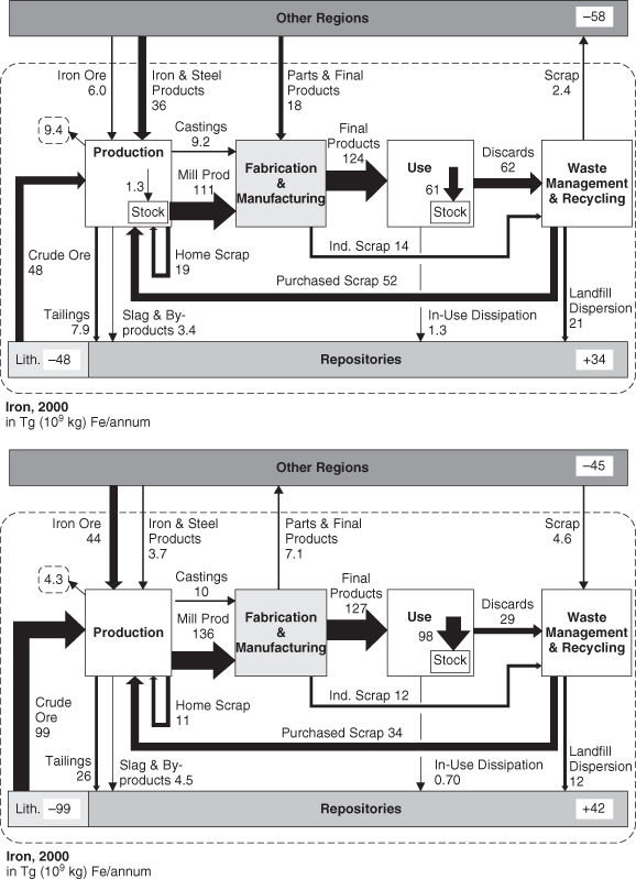
While Figure 4-7 characterizes the flows of iron on a global basis, flows of materials can vary among regions. Mapping regional flows requires the addition of flows from other regions and to other regions (exports and imports); these flows are not required for a global material balance. As an example, Figure 4-8 compares the flows of iron in the United States and China. The United States uses a larger fraction of recycled iron than China.
Figure 4-8. Flows of iron in the United States and China, 2000 (Wang et al., 2007; reprinted with permission, STAF Project, Yale University)
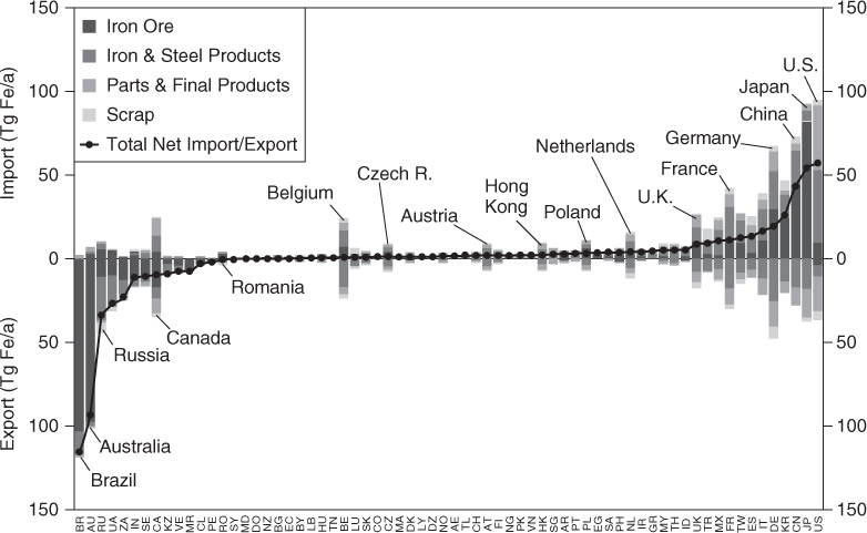
Understanding the sourcing of materials, and the geopolitical issues associated with source regions, will become increasingly important as global demands on resources increase. Figure 4-9 shows the extent to which various countries are net importers or exporters of iron. The world’s leading exporter of iron is Brazil, and the leading importer (for both total imports and net imports [imports-exports]) is the United States. Countries such as Belgium, the Netherlands, and the United Kingdom are both importers of iron as a raw material and exporters of iron in manufactured goods.
Figure 4-9. Importing and exporting of iron, by country, ranked by net imports minus exports (Reprinted with permission from Wang et al., 2007. Copyright 2007, American Chemical Society)
The case of iron is not unusual. Global trade in commodity materials leads to some countries becoming net importers, while others are net exporters, depending on the material. For example, while China is a net importer of iron, it is a dominant producer and exporter of rare earth metals.
Combinations of materials scarcity, potential energy savings, and geopolitical factors may lead to increased rates of recycling and reuse for many materials. A qualitative indicator of the potential for such recycling to occur is once again the Sherwood diagram. In Figure 4-3, dilution in virgin ores was shown to be a reasonable predictor of price for many materials. Another way in which this diagram can be used is to assess the degree to which waste streams might be “mined.” Allen and Behmanesh (1994) examined the extent to which hazardous wastes in the United States might be mined (cost-effectively recycled) by comparing the degree of dilution of metals in hazardous waste streams to commodity prices. Their original analysis, summarized in Table 4-3, found that many hazardous waste streams in the United States had high enough concentrations of metals to merit additional recycling. Hazardous wastes were chosen because detailed data existed on their compositions, flow rates, and fates. Surprisingly, many hazardous waste streams contain relatively high concentrations of metals. Approximately 90% of the copper and 95% of the zinc found in hazardous wastes were, at the time, at concentrations high enough to recover. For every metal for which data existed, recovery occurred at rates well below rates that would be expected to be economically viable.
Table 4-3. Percentage of Metals in Hazardous Wastes in the United States That Can Be Recovered Economically
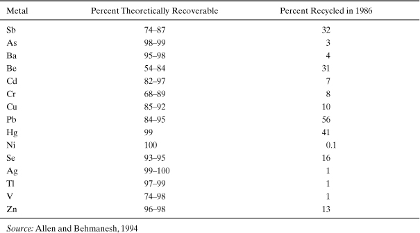
This very focused analysis, which was initially performed in 1994 (Allen and Behmanesh, 1994), led to the conclusion that many opportunities existed for recovering materials from wastes. There are limitations to the analysis, however. The analysis focused only on hazardous wastes, where legal liability concerns may limit the desire to recycle. The identification of “recyclable” streams was simplistic. It ignored issues related to economies of scale (i.e., processing geographically dispersed, heterogeneous waste streams may be more expensive than extracting a relatively homogeneous ore from a single mine). Nevertheless, the analysis indicated that resources are not effectively recovered from many waste streams.
The United Nations has assembled more recent, global data on metals recycling. Its analysis continues to conclude that global recycling rates can continue to be improved. Metals like Pb (along with Fe, Cr, Co, Ni, Cu, Zn, and many precious metals) have postconsumer recycling rates that exceed 50% globally, but many other metals (e.g., rare earth elements) have postconsumer recycling rates of less than 1% (United Nations Environment Programme, 2011).
One of the primary barriers to using wastes as raw materials is a lack of critical information on waste streams. While a large number of data sources are available on waste streams, they lack critical information that is needed to assess whether the waste streams might be reused. Data on the composition of wastes, their location, and co-contaminants are rarely available yet are critical to evaluating the potential use of wastes as raw materials.
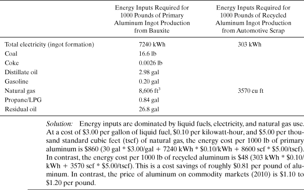
Example 4-7. Energy savings due to recycling
Aluminum is extensively recycled, in part because of the energy savings associated with reprocessing recycled aluminum into aluminum stock, as compared to the processing of bauxite into aluminum. The table below shows the differences in fuel and electricity inputs required for primary aluminum (from bauxite) and aluminum recycled from automotive scrap (U.S. Life Cycle Inventory data available at www.nrel.gov/lci). Using current prices for the fuels and electricity, calculate the differences in energy costs, per pound of aluminum. How does this compare to the market price of aluminum?
To summarize, material flow tracking can identify overall availability of materials and potential opportunities for material reuse or recycling. One way to view these flows is as an opportunity to change the designs of industrial systems so that they more closely resemble highly networked, mass-conserving, natural ecosystems, an industrial ecology. As this text is being written, the data necessary to perform detailed material tracking are just beginning to emerge in a consistent framework. For many analyses, it will be necessary to assemble the necessary data on material use and flows on a case-specific basis. Nevertheless, these types of analyses will become increasingly valuable as material scarcity becomes an important issue.
4.4. Environmental Releases
A material, at the end of its useful life cycle or as a consequence of its production or use, is released into the environment. Will its release pose significant environmental or human health risks? Will the chemical degrade in the environment or will it persist?
The challenges involved in answering these questions are formidable. Tens of thousands of chemicals are produced commercially, and every year, a thousand or more new chemicals are developed and introduced into commerce. For any chemical in use, there are a number of potential risks to human health and the environment. In general, it is not practicable to rigorously and precisely evaluate all possible environmental impacts. Nevertheless, a preliminary screening of the potential environmental impacts of chemicals is necessary and is possible. Preliminary risk screenings allow businesses, government agencies, and the public to identify problem chemicals and to identify potential risk reduction opportunities. The challenge is to perform these preliminary risk screenings with a limited amount of information.
The goal of this section is to describe qualitative and quantitative methods for estimating environmental risks when the only information available is a chemical structure. Many of these methods have been developed by the U.S. EPA and its contractors. The methods are routinely used in evaluating Premanufacture Notices (PMNs) submitted under the Toxic Substances Control Act (TSCA). Under the provisions of TSCA, before a new chemical can be manufactured in the United States, a PMN must be submitted to the EPA. The notice specifies the chemical to be manufactured, the quantity to be manufactured, and any known environmental impacts as well as potential releases from the manufacturing site. Based on these limited data, the EPA must assess whether the manufacture or use of the proposed chemical may pose an unreasonable risk to human or ecological health. To accomplish that assessment, a set of tools has been developed that relate chemical structure to potential environmental risks.
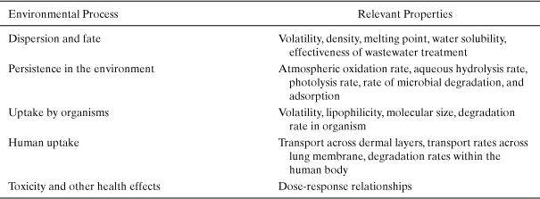
Table 4-4 identifies the chemical and physical properties that will influence the processes that determine environmental exposure and hazard. The table makes clear that a wide range of properties needs to be estimated to perform a screening-level assessment of environmental risks.
Table 4-4. Chemical Properties Needed to Perform Environmental Risk Screenings
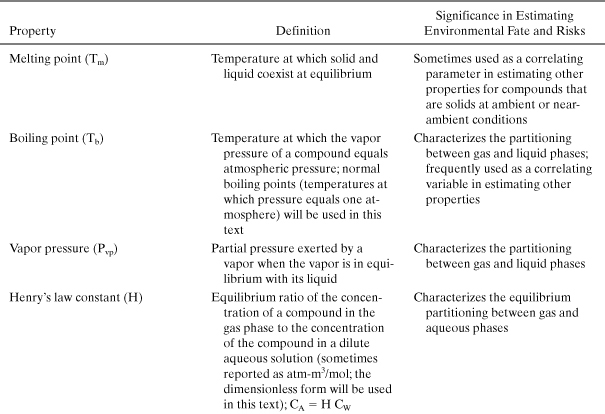
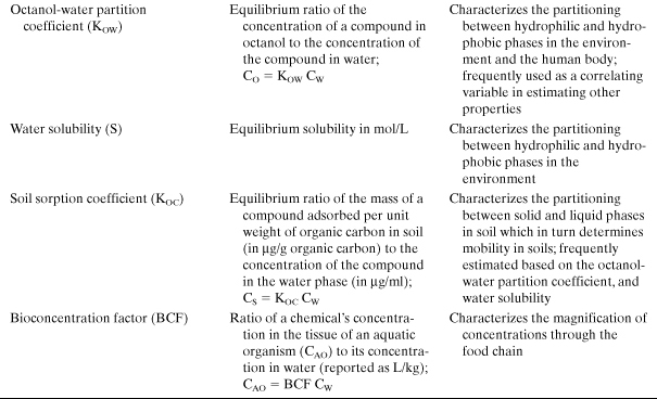
The first group of properties that must be estimated in an assessment of environmental risk are the basic physical and chemical properties that describe a chemical’s partitioning among solid, liquid, and gas phases. These properties are important in determining whether a pollutant will concentrate in air, water, soil, or living organisms and include melting point, boiling point, vapor pressure, and water solubility. Additional molecular properties, related to phase partitioning, that are frequently used in assessing the environmental fate of chemicals include the octanol-water partition coefficient, soil sorption coefficients, Henry’s law constants, and bioconcentration factors. (Each of these properties is defined in Table 4-5.) Once the basic physical and chemical properties are defined, a series of properties that influence the persistence of chemicals in the environment are estimated. These include estimates of the rates at which chemicals will react in the atmosphere, the rates of reaction in aqueous environments, and the rates at which the compounds will be metabolized by organisms. If environmental concentrations can be estimated based on release rates and environmental fate and persistence properties, human exposures to the chemicals can be estimated. Finally, if exposures and hazards are known, risks to humans and the environment can be estimated.
Table 4-5. Properties That Influence Environmental Phase Partitioning
These chemical and physical properties can be used to evaluate a variety of metrics related to environmental impacts; some of the most commonly evaluated environmental metrics are persistence, bioaccumulation, and toxicity. For any one of these metrics of environmental impact, it may be necessary to consider a number of properties in performing an evaluation. For example, in evaluating persistence, atmospheric half-lives and biodegradation half-lives may be needed. In evaluating toxicity, it may be necessary to consider a variety of ecotoxicity measures and human toxicity measures. Because there is such a wide variety of criteria that can be used in evaluating environmental risks—ranging from human carcinogenicity to biodiversity—and because opinions vary widely on the relative importance of the evaluation criteria, there is no single evaluation methodology that is universally accepted for evaluating the environmental hazards of chemicals.
While it is not the only approach, measures of persistence, bioaccumulation, and toxicity are used by the EPA in evaluating PMNs under TSCA, and in performing these evaluations, the EPA classifies chemicals into categories of high, moderate, and low concern. Methods for estimating persistence, bioaccumulation, and toxicity rely on estimates of physical and chemical properties, such as those listed in Tables 4-4 and 4-5. Methods for estimating these properties are described by Allen and Shonnard (2001), and the impact of the properties on assessing environmental persistence and fate is presented in problems at the end of this chapter.
4.4.1. Using Property Estimates to Evaluate Environmental Partitioning, Persistence, and Measures of Exposure
This section will briefly illustrate, through examples, how chemical and physical properties can be employed to estimate environmental partitioning, persistence, and measures of exposure. The problems associated with estimating environmental exposures are complex. Consider the relatively simple example of calculating exposure through drinking contaminated surface water. Assume that a chemical is released to a river upstream of the intake to a public drinking water treatment plant. To evaluate the exposure we would need to determine
• What fraction of the chemical was adsorbed by river sediments
• What fraction of the chemical was volatilized to the atmosphere
• What fraction of the chemical was taken up by living organisms
• What fraction of the chemical was biodegraded or was lost through other reactions
• What fraction of the chemical was removed by the treatment processes in the public water system
In this case, exposure estimates will require information on the soil sorption coefficient, vapor pressure, water solubility, bioconcentration factor, and biodegradability of the compound, as well as river flow rates, surface area, sediment concentration, and other parameters. Often, for screening calculations, equilibrium partitioning of compounds is assumed between water and soil, water and air, and water and living systems. Assuming equilibrium partitioning allows ratios of concentrations to be determined. For example, the Henry’s law coefficient defines the equilibrium ratio of air and water concentrations. The soil sorption coefficient allows equilibrium ratios of soil and water concentrations to be determined, and bioconcentration factors determine the ratio of biota and water concentrations. A simple, yet typical, set of calculations is shown in Example 4-8.
Example 4-8. Environmental Partitioning
Assume that a chemical with a molecular weight of 150 is released at a rate of 300 kg/day to a river, 100 km upstream of the intake to a public water system. Estimate the initial equilibrium partitioning of the chemical in the water, sediment, and biota.
Data: Soil sorption coefficient: 10,000 (ratio of concentration of pollutant in soil to the concentration in water)
Organic solids concentration in suspended solids: 15 ppm
River flow rate: 500 million L per day
Bioconcentration factor: 100,000 (ratio of concentration of pollutant in biota (fish) to the concentration in water)
Biota loading: 100 g per 100 cubic meters
Solution: The ratio of concentrations in water, sediment, and biota will be approximately
1 : 10,000 : 100,000
Based on the river flow rate, the total flow rates of water, sediment, and biota are
Water: (500 million L/day * 1 kg/L) = 500 million kg/day Sediment: 500 million kg/day * 15 kg sediment/million kg water = 7500 kg sediment/day
Biota: 500 million kg/day * 0.1 kg biota/million kg water = 50 kg biota/day
Performing a mass balance:
300 kg/day = 500 million kg water/day (Cwater)+ 7500 kg sediment/day (10,000 Cwater) + 50 kg biota/day (100,000 Cwater)
where (Cwater) is the chemical concentration in the water phase,
(Cwater) = 0.5 * 10-6 kg chemical/kg water = 0.5 ppm
Concentration in sediment = 0.5 ppm * 10,000 = 5000 ppm
Concentration in biota = 0.5 ppm * 100,000 = 50,000 ppm
The ratio of the mass in water, sediment, and biota is
500,000,000 : 7500 (5000) : 50 (50,000)
84 : 13 : 1
Thus, although the concentrations are much higher in the biota and the sediment phases, more than 80% of the mass remains in the water phase.
4.4.2. Direct Use of Properties to Categorize the Environmental Risks of Chemicals
Section 4.4.1 illustrated how chemical and physical properties can be used to estimate environmental footprints. Another approach is to use the values of properties to directly categorize the environmental risks of chemicals. For example, Table 4-6 is a summary of the categories used by the EPA to classify the persistence and bioaccumulation of chemicals.
Table 4-6. Classification Criteria for Persistence and Bioaccumulation
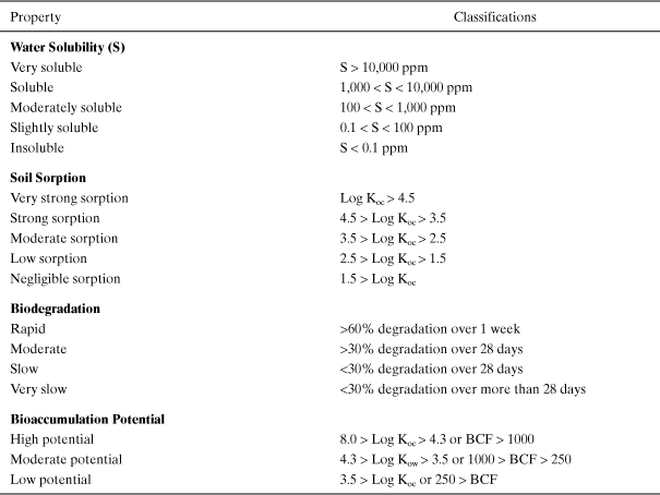
For each of these categories, a score might be given. For example, persistence might be scored 1 through 4 for the four levels of biodegradation listed in Table 4-6. Bioaccumulation might be given a score of 1 through 3 based on the three categories of bioconcentration factor. Similar scores could be developed for toxicity. These indices or scores could then be combined, for example, by adding the scores, to arrive at a composite index.
Other categories could be used to classify materials. Example 4-9 compares a variety of chemicals used in fuels.
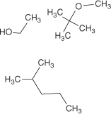
Example 4-9. Classifying fuel molecules
Compare the soil sorption, water solubility, and biodegradation of three compounds that have been used in gasoline: ethanol, methyl-tert butyl ether (MTBE), and isohexane. Use these data to assess which of the chemicals, if spilled on land, would be more likely to migrate to surface or groundwater. Isohexane is one of the most commonly found molecules in gasoline derived from petroleum. Ethanol is commonly obtained from corn grain, and MTBE was produced in large quantities in the United States from methanol (derived from natural gas) and light petroleum gases (isobutylene).
Solution: Properties for these compounds can be determined through property databases or using methods described in Allen and Shonnard (2001).
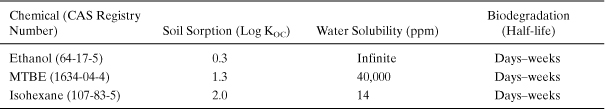
The results indicate that petroleum-derived gasoline, if spilled onto ground, is more likely to adsorb to soils than MTBE and ethanol, making it less likely to migrate to water sources and cause water contamination. In contrast, however, MTBE and ethanol have been added to gasoline because of provisions of the Clean Air Act that are designed to reduce emissions of air pollutants. So, while ethanol and MTBE are more likely to find their way into surface and groundwaters than components of conventional gasoline, their use can improve air quality.
4.5. Summary
Almost every engineering design involves the use of materials, and these materials have environmental footprints. Methods for characterizing the footprints associated with extraction, processing, and environmental releases of materials have been described in this chapter, but these assessments can lead to very different characterizations of materials. Is the material scarce? Can it be recycled? Do environmental releases have significant impacts?
There are no universally accepted methods for combining these characterizations of whether a material is sustainable. Multiple methods are used. Engineers will need to consider materials in the context of particular designs, recognizing that the choice of the most sustainable materials will be application-specific.
Problems
1. Material use in photovoltaic manufacturing Approximately 65 gigawatts of electrical power are consumed during periods of peak demand in Texas. If the entire demand were to be met by copper-indium-gallium-diselenide (CIGS) photovoltaic cells requiring 50 kg of indium and 10 kg of gallium per megawatt of power generated, calculate the total amounts of Ga and In required to manufacture these cells, and compare these quantities to the total worldwide production of Ga and In (see U.S. DOE, 2010).
2. Materials use in wind turbine manufacturing Approximately 65 gigawatts of electrical power are consumed during periods of peak demand in Texas. If the entire demand were to be met by wind power, and the wind turbines require 25 kg of dysprosium per megawatt of power generated, calculate the total amount of Dy required to manufacture these turbines, and compare this quantity to the total worldwide production of Dy (see U.S. DOE, 2010).
3. Recycling rare earth elements from hybrid vehicles Estimate the potential flow of recycled rare earth elements that could be recovered from plug-in hybrid electric vehicles (PHEVs) by 2030. Assume that 10 kg of rare earth elements are used in a typical PHEV and that, by 2030, 5 million vehicles per year are retired and available for recycling. Compare the potential flow of recycled material to current mine production.
4. Ranking critical materials The U.S. Department of Energy has used a method for categorizing critical materials that involves plotting the ranking of both the supply and the potential demand, where demand includes assessments of both the growth in markets for products and the development of alternative materials. Select one of the materials from the Department of Energy assessment and write a one-page summary describing the basis for the rankings (U.S. DOE, 2010).
5. Materials use in green products The EPA has developed a Design for Environment labeling program for a variety of products. Visit the Web site for the program and write a one-page summary of the criteria used in awarding the Design for Environment label (www.epa.gov/oppt/dfe/index.htm or www.epa.gov/oppt/dfe/pubs/projects/gfcp/index.htm#Standard).
6. Environmental fate of gasoline substitutes The compound methyl-tert butyl ether (MTBE) has been used extensively as a gasoline additive. If 100 kg of this compound were accidentally spilled into a lake over the course of a summer, calculate the concentrations in water, sediment, and fish (neglect volatilization) that would result. Assume that the volume of the lake is 8 * 107 m3, the organic solids loading is 20 ppm, and the fish loading is 2 kg per 104 m3. Assume that the lake is well mixed.
a. What are the concentrations in water, sediment, and fish?
b. What fraction of the MTBE would be found in the sediment?
c. What fraction would be found in the fish?
d. If you swallowed 1 L of water during a day while waterskiing, how much MTBE would you ingest?
Soil adsorption coefficient: 11.56 L/kg
Bioaccumulation factor: 3.162 L/kg wet-wt
7. Environmental fate of medications Medications can enter wastewater management systems either through human excretions or through improper disposal. Many medications are not effectively treated by current wastewater management processes and therefore are discharged by wastewater treatment plants. Antidepressants are some of the most commonly prescribed medications in the United States, and many antidepressants are not effectively managed by wastewater treatment plants.
a. A wastewater treatment plant discharges to Boulder Creek in Colorado at a rate of 64 million L/day, and the stream flow, upstream of the wastewater discharge point, is 1110 L/s. If the concentration of the antidepressant venlafaxine (Effexor) measured in the creek water is 10 ng/L, what is the mass discharged per day from the wastewater treatment plant, assuming that there are no sources other than the wastewater treatment plant, and assuming that the drug rapidly equilibrates among sediment, fish, and water? What is the concentration of the medication in the wastewater treatment plant effluent?
BCF = 40.27
KOC = 3.162
Organic sediment = 15 ppm
Biota concentration = 5 g/100 m3
b. A man fishing near the outflow point of Boulder Creek eats 0.2 kg of fish from the creek. How much venlafaxine will he ingest? One dose of Effexor contains 75 mg of venlafaxine. What percentage of a dose will the fisherman ingest?
References
Allen, D. T. 1996. “Waste Exchanges and Material Recovery.” Pollution Prevention Review 6(2):105–12.
Allen, D. T., and N. Behmanesh. 1994. “Wastes as Raw Materials. In The Greening of Industrial Ecosystems, edited by B. R. Allenby and D. J. Richards. Washington, DC: National Academy Press, pp. 69–89.
Allen, D. T., and D. R. Shonnard. 2002. Green Engineering: Environmentally Conscious Design of Chemical Processes. Upper Saddle River, NJ: Prentice Hall.
Gerst, M., and T. E. Graedel. 2008. “In-Use Stocks of Metals: Status and Implications.” Environmental Science & Technology 42:7038–45.
Graedel, T. E., and B. R. Allenby. 1995. Industrial Ecology. Englewood Cliffs, NJ: Prentice Hall.
Johnson, J., E. M. Harper, R. Lifset, and T. E. Graedel. 2007. “Dining at the Periodic Table: Metals Concentrations as They Relate to Recycling.” Environmental Science & Technology 41:1759–65.
Kesler, S. E. 1994. Mineral Resources, Economics and the Environment. New York: Macmillan.
National Research Council. 2003. Materials Count. Washington, DC: National Academy Press.
Taylor, S. R. 1964. “Trace Element Abundances and the Chondritic Earth Model.” Geochimica et Cosmochimica Acta 28(12):1989–98.
United Nations Environment Programme. 2011. Recycling Rates of Metals: A Status Report. Available at www.unep.org/resourcepanel/Publications/Recyclingratesofmetals/tabid/56073/Default.aspx. Accessed July 2011.
U.S. DOE (U.S. Department of Energy). 2010. Critical Materials Strategy. December. Available at www.energy.gov/news/documents/criticalmaterialsstrategy.pdf.
USGS (United States Geological Survey). 2000. Materials and Energy Flows in the Earth Science Century. Circular 1194.
___________. 2010. Mineral Commodities Summaries. Washington, DC: U.S. Government Printing Office.
Wang, T., D. B. Müller, and T. E. Graedel. 2007. “Forging the Anthropogenic Iron Cycle.” Environmental Science & Technology 41:5120–29.