
8
Comparative Wear Model on Hybrid Natural Fiber Composites as Substitutions for UHMWPE Made Knee Implants
Gusztáv Fekete and Mátyás Andó
Eötvös Loránd University, Faculty of Informatics, Savaria Institute of Technology, Szombathely, H‐9700, Hungary
8.1 Introduction
8.1.1 Basics of Reinforced Polymers, Composites, and Their Testing
Engineering materials have undergone a great evolution in history. Depending on the technology available at a given time, certain preferences were made for materials as well. This relative importance of materials is seen in Figure 8.1. As is seen, due to the work and success of material researchers, more and more new polymer and composites materials have been developed in the last decades.

Figure 8.1 The relative importance of the materials in the history.
Source: Ashby 2009 [1]. Reproduced with permission from Elsevier.
Besides polymers, hundreds of new materials exist with regard to ceramics or metals. As a result, traditional classifications – metal, polymer, ceramic, and composites – changed to application based classifications (aerospace materials, electronic materials, smart materials, etc.). To understand hybrid natural fiber composites (NFCs) better, a brief introduction about polymers is necessary.
8.1.2 Classification of Polymers
The industrial history of polymers started with rubber in the twentieth century. The first spurt in the application of different polymers was around the time of the Second World War. For the last 20–30 years the applications and the types of polymers increased continuously. It must be noted that polymers can be synthetic or natural, but this classification only refers to the source, not to the structure.
Polymers are organic materials that have specific macromolecular structures. Monomers are the basic units, which can repeat 10 000 times in a single polymer chain. The simplest monomer is ethylene (C2H4), which has double bonds between carbon atoms.
The following chemical process has to be carried out in order to create a simple polymer chain: the double bonds connecting two neighboring monomers must be broken first, and a new single bond connection must be created (Figure 8.2) to achieve a chain.

Figure 8.2 Ethylene monomers before and after the reaction and their symbolic representation.
There are thousands of monomers that create different macromolecular structures as well. Based on these structures the polymers can be thermoplastics or thermosets. The basic difference between the two structures is the cross‐link. In the case of thermoplastics there are no cross‐links between the chains (Figure 8.3a); therefore, these materials can remold after solidification. The thermosets have cross‐links; thus during the chemical reaction when they are formed, they cannot be remolded any more (Figure 8.3b).

Figure 8.3 Structures of thermoplastics (a) and thermosets (b).
In thermoplastic structures, there are only secondary chemical bonds between the polymer chains. If the temperature rises to a limited point, the secondary chemical bonds break and the polymer chains can slip next to each other. Primary chemical bonds need much more energy to break so that the polymer chains could remain complete. After cooling, the new position of the chains becomes fixed by the new secondary chemical bond. Thermosets cannot melt since there are only primary chemical bonds in their structure. At much higher temperatures, both the chain and the cross‐link can be broken.
Naturally, in this elevated temperature the thermoplastic is also degraded, but there is still a technological range in the temperature where they can melt and a new shape can be created (by injection molding, extrusion, etc.).
Thermoplastic polymers have two different subtypes in their structures. If the molecules solidify in a random arrangement, then the polymers become amorphous (Figure 8.4a). Amorphous thermoplastics are generally transparent. If polymer chains show some dimensional order locally, then they are called semi‐crystalline polymers (Figure 8.4b).

Figure 8.4 Structure of amorphous (a) and semi‐crystalline polymers (b).
The degree of crystallinity is one of the important parameters that have direct connection to the material property of the polymer. The degree of crystallinity can vary from 1% to 100%.
Thermoset polymers have cross‐links between the chains that provide better heat resistance. Based on the amount of cross‐links two groups can be differentiated: slightly cross‐linked thermosets or elastomers (e.g. rubber) and highly cross‐linked thermosets or duromers (e.g. epoxy resin).
8.1.3 Classification of Composites
Composites have different definitions. Nowadays, if a material has at least two additives, then companies in material science business term it a “composite,” but mostly this is only for marketing reasons. The polymer industry uses the so‐called fillers since the beginning of material production. Originally, if a filler can reinforce the polymer and improve its mechanical performance, then it can be a composite. In the case of polymers, the most typical reinforcing material is probably glass fiber, and it is widely used in thermoplastics and thermosets as well.
Fibers mostly have improved mechanical behaviors than the polymer (matrix). The purpose of the fiber is to make stronger connection between two neighboring areas in the material. Here, something must be made clear. In engineering, Young’s modulus is likely the most important parameter, rather than tensile strength. If the material has high modulus, then the resistance of the deformation is also high (high stiffness). This consideration is the main theory behind reinforced composites. Fibers also have the role of transferring load if they have appropriate connection with the matrix. The fibers connect to the matrix through chemical adhesion. If the adhesion is strong enough, then the composite will have adequate stiffness as well. If the adhesion is low, the fibers tend to loosen (pull out) and they create a dramatic decrease in the stiffness (Figure 8.5).

Figure 8.5 Composite behavior in case of different adhesion.
If the matrix has only one fiber reinforcement, the maximum effect can only be achieved if the fiber breaks (tensile strength – σ). This also means that the adhesion must be strong enough, which depends on the surface and the shear strength (τ) of the fiber–matrix connection. Based on a mechanical equation (if the fiber has perfect cylindrical surface) the critical length (Lc) can be calculated:
If the fiber is longer than the critical length, then it works effectively. In many cases, it is easier to achieve shorter fibers, which also makes working with it easier (e.g. injection molding), than enhancing the chemical adhesion to a higher level. There are different treatments to achieve better chemical connections that can improve the shear strength between the fiber and the matrix.
If the fiber is long enough and the deformation remains in the linear region of the material, then Hooke’s law can be applied with regard to the parallel fibers:
where Ec is the Young’s modulus of the composites, Ef is the Young’s modulus of the fiber, Em is the Young’s modulus of the matrix, and Vf is the volume of the fiber. To achieve real reinforcement by applying fibers, usually the Young’s modulus and the tensile strength must be kept relatively high while the density is low. Table 8.1 includes some typical fibers used for reinforcement and their properties [2].
Table 8.1 Typical fibers for reinforcement use.
| Fiber type | Density (g cm−3) | Tensile strength (GPa) | Young’s modulus (GPa) |
| Steel | 7.86 | 4.0 | 210 |
| Glass fiber (E‐type) | 2.6 | 2.5 | 72 |
| Carbon fiber (HS) | 1.78 | 3.4 | 240 |
| Aramid (Kevlar 49) | 1.44 | 3.3 | 75 |
| Polyethylene (SK 66) | 0.97 | 3.3 | 99 |
Different plants or animals form the source of natural fibers. It is generally true that these fibers are biodegradable and they are from renewable sources. Table 8.2 lists some typical natural fibers and their properties [3].
Table 8.2 Typical natural fibers.
| Fiber type | Density (g cm−3) | Tensile strength (GPa) | Young’s modulus (GPa) |
| Bamboo (manual extraction) | 0.91 | 0.5 | 35.9 |
| Palm | 1.03 | 0.4 | 2.7 |
| Coconut | 1.15 | 0.5 | 2.5 |
| Banana | 1.35 | 0.6 | 17.9 |
| Sisal | 1.45 | 0.6 | 10.4 |
Composite materials can be classified according to their length and their orientation. Based on the length, there are two types: short fiber/discontinuous fiber (longer than the critical length) and continuous fiber (c. thousand times longer than the critical length). The orientations are also of two types: random (fibers have different directions) and aligned (all the fibers are in the same direction).
In two dimensions (sheet forms), there can be continuous aligned structures (Figure 8.6a), short aligned structures (Figure 8.6b), short random structures (Figure 8.6c), and continuous random structures (Figure 8.6d). In addition, different fiber weaves/fabrics also exist (Figure 8.6e).
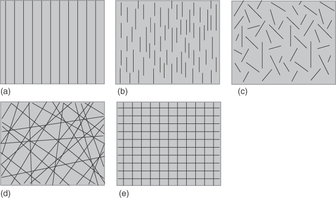
Figure 8.6 (a–e) Different composite structures in two dimensions.
Composite structures can be more complex in three dimensions. Depending on the technologies, usually there are more layers laid on each other. 2D aligned structures become random structures if the different layers have free directions. It must be noted that 3D fabrics exist that have oriented structure in 3D as well. These types of structures allow engineers to design composite parts where the reinforcement completely fits the stress distribution and the directions.
Additional need for optimizations and special properties led the researchers in composite technology to create innovative solutions. Hybrid composites are an answer to this need. Hybrid composites contain at least two types of fibers, where the different fibers can be in the same sheet (2D), or the different layers can create a hybrid system in 3D.
8.1.4 Basics of Tribo‐testing
Tribology is a science that deals with friction, wear, and lubrication. In reality, two interacting surfaces create a complex phenomenon with regard to tribology. In order to obtain a clear view about this contact phenomenon in relation to tribological behaviors, a schematic tribological system was created (Figure 8.7).

Figure 8.7 Simplified tribological system.
Basically, all tribological systems include two bodies, the motion of which can be described with the law of relative kinematics. Usually, the intermediate material plays the role of a lubricant and the wear debris. The rest of the parameters (e.g. temperature, load, sliding distance, surface roughness, materials) belong to the tribological environment. During an experiment, the researchers attempt to identify the main parameters and to be able to control them in the future experiments. One of the basic equations in tribology is the ratio of the coefficient of friction:
where FF is the friction force and FN is the normal force. Both the friction force and the normal force are influenced by many parameters that are included in the tribological environment. Owing to these parameters and their statistical deviance, high deviations are expected during repeated tribological measurements, even though the parameters are seemingly fixed. Figure 8.8 contains the classification of tribo tests.

Figure 8.8 Classifications of tribo tests.
Source: Bhushan 2001 [4]. Reproduced with permission from CRC Press.
Tests can be performed in almost endless number of ways. Typical factors are running time, accurate control of test conditions, isolated wear mechanisms, and so on. Generally, a test model is used to better identify the main tribological behavior. Testing a simplified model is considerably easier, quicker, and cheaper under well‐controlled test conditions, but it also correlates less with reality. Creating an appropriate model to address a real tribological problem is probably the most challenging part of the research. Researchers need to deal with basic effects (approximately the seven more important ones) to simulate the tribological conditions.
These effects are as follows:
- Contact (tribocouples: ball on plate, block on ring, block on plate, pin on disk, etc.)
- Load (forces, Hertzian contact, etc.)
- Displacement (sliding, rolling, spinning, flowing, oscillating, impact, etc.)
- Relative motion (constant, periodical, magnitude, etc.)
- Track (clean surface, transfer film, lubrication, debris, etc.)
- Surface roughness (Ra, Rz, etc.)
- Temperature
Based on the earlier results, typical wear and friction models have been already established. The principle wear mechanisms are recognized as adhesive wear, abrasive wear, erosive wear, corrosive wear, and fatigue wear. Mostly, the wear debris changes the tribological environment by altering its complexity and deviations. In addition, in real applications there are no clear conditions that bring forth more complex wear phenomena.
8.1.5 Hybrid Natural Fiber Composites and Their Possible Use in Total Knee Replacements (TKR)
As was mentioned earlier, fibers are mostly classified based on their source, which can be related to minerals, plants, and animals. Biologically, these materials are made up of either cellulose or proteins depending on the source. Lately, there has been a rapid growth in R&D in the NFC area.
The particular interest in this material is due to the advantages in their mechanical properties compared to synthetic fiber composites, not mentioning the low environmental impact cost as well. It must be also mentioned that usually higher performance can be credited to plant fibers than the available animal fibers with regard to their higher strengths and stiffness.
Among the numerous possible applications, companies involved in biomedical part production are also interested in this new type of materials as a possible substitution for UHMWPE manufactured elements. Naturally, these new materials can only enter the market if they are able to provide acceptable wear characteristics and resilience compared to the materials being used today.
Undeniably, problems related to wear in total knee replacements (TKRs) have decreased in the past 10 years [5] but not disappeared. In the design‐related factors, wear is still the second most important mechanical factor (first is the periprosthetic fracture) that limits the lifetime of TKRs and it also greatly depends on the local kinematics of the knee.
On studying the wear properties of these materials, it becomes quite evident that NFCs have significant difference in their wear behavior. An important parameter that is widely used in analytical and numerical modeling is the specific wear coefficient (denoted as k), which is summarized in Table 8.3.
Table 8.3 Specific wear coefficient in case of natural fibers.
| Author | Material | Load (N) | Velocity (mm s−1) | Specific wear coefficient (mm3 N−1 m−1) |
| Chittaranjan and Acharya [6] | Lantana camara | 20 | 31.4 | 1.5 × 10⁻¹¹ |
| Ren et al. [7] | Hybrid PTFE | 20 | 26 | 1.4 × 10⁻¹⁴ |
| Omrani et al. [8] | Jute | 20 | 30 | 4 × 10⁻⁷ |
| Yousif et al. [9] | Palm fiber reinforced polyester | 20 | 30 | 2.5 × 10⁻⁶ |
| Patten et al. [10] | UHMWPE against CoCr | 200 | 30 | 1.3 × 10⁻⁶ |
It must be also noted that these materials were tested approximately with the same sliding speed, but the load is significantly less than in the study by Patten et al. [10], where the authors tested materials that are actually being used in TKR production.
By looking at these results, it is apparent that the specific wear coefficient of the Lantana camara and the hybrid PTFE are exceptional, but it is unknown yet whether they could perform as well as the UHMWPE if the load is elevated not only to 200 N but significantly beyond. The palm fiber reinforced polyester is in the same range regarding the specific wear coefficient compared to the standard UHMWPE materials used in TKRs.
Since the load in the TKR can be up the six to seven times the body weight (BW) during squatting and two to three BW during gait, more experimental data are needed before these materials could enter the market not only as substitutional choices but also as prime material possibilities.
8.2 Aims
In this chapter, the main aim is to introduce an enhanced wear model that can be a useful tool for estimating wear outcome for NFCs, if the specific wear coefficient is available. As a first step, a classical UHMWPE material is chosen to give an insight on how the analytical wear model works if knee‐specific parameters such as the slide–roll ratio or the varying load in case of non‐standard and standard squat are incorporated into it.
As for wear in knee implants, it must be noted that this phenomenon is, on one hand, caused by the non‐congruent form of the knee joint together with its natural instability. On the other hand, emerging particle debris can also be a relevant cause of cartilage damage. Nevertheless, it must be pointed out that the phenomenon of wear is in relation with several interrelated factors; thus, it must be examined as a system, not as a material property [11].
Wear is the second among the main mechanical factors that limit the lifetime duration of TKRs [5, 12, 13] and it is also highly dependent on the kinematics of the knee joint [14]. Beside multiple other parameters in wear studies, slide–roll ratio between 0% and 40% is frequently applied during tribological tests carried out with pin‐on‐disk test rigs or knee simulators [15, 16]. During wear tests, its magnitude is always considered constant based on the study of McGloughlin and Kavanagh [17] and Hollman et al. [18]. This approximation is correct if it is applied on pin‐on‐disk or ball‐on‐disk tests, where the kinematics is precisely adjusted to this special configuration.
Nevertheless, several authors published results that are against the idea of constant slide–roll ratio regarding TKRs [19, 20] where they referred to the complex geometry, which highly alters the local kinematics. It was demonstrated in the study of Laurent et al. [21] that the wear mechanism is highly dependent not only on the load in the contact but also on the interfacial contact kinematics, which includes a cyclic multidirectional path of motion and the slide–roll ratio.
Thus, varying the slide–roll ratio under the different motions (gait, squat, etc.) can be a possible parameter to give a better approximation on TKR wear mechanism.
In the following, a more realistic mathematical approach on wear propagation between the tibiofemoral connections will be introduced. For the analysis, a commonly applied wear model, Archard’s equation, is used [22], which incorporates the friction force, derived from the tibiofemoral force in the contact, with a varying slide–roll ratio.
In spite of its simplicity, Archard’s equation is widely used in the contemporary literature [23, 24] and the predicted wear is in reasonable agreement with other more sophisticated models such as the model of Turel et al. [25] or the model of Abdelgaied et al. [26]. Squat is chosen for analyses regarding wear, since during this motion the highest contact forces [27] and the highest slide–roll ratio can be approached [20]. Along with the abovementioned fact, squat is a widely exercised movement for rehabilitation and for thigh muscles strengthening due to sport or medical reasons [28, 29]; therefore, it is important to know the aspect of wear with regard to this motion.
8.3 Methods
8.3.1 Wear Modeling
The instantaneous volume of material removed from the tibiofemoral surface of the TKR due to mild wear is predicted by Archard’s law [22]:
where k is the specific wear rate (mm3 N−1 m−1), which is a material‐dependent quantity; FN is the normal force acting between the contact surfaces, which in this case is the contact surface of the tibia and the femur (N); and ds is the infinitesimal length of sliding (m). There are two parameters in this equation that are to be further enhanced: the force and the sliding length wherein the slide–roll ratio can be defined.
The wear mechanism between the connecting surfaces is supposed to be abrasion based (two‐body). This means that during contact, the harder metallic femoral part ploughs into the softer polyethylene tibial part, and in the connecting point(s) reaction force(s) appear (Figure 8.9). As a first step, we can approximate these forces with the Coulomb law:
Figure 8.9 Two‐body abrasive wear between the connecting surfaces.
where μk is the coefficient of kinetic friction.
In the abrasive wear mechanism, the frictional component is responsible for creating such a shear stress in the upper surface of the material that it begins to lose small debris. Therefore, it provides us a more precise approximation if the friction force, deduced from the tibiofemoral force, is introduced in our wear equation:
8.3.2 Force Modeling for Wear Equation
The normal force in Equation (8.6) that acts between the connecting surfaces is considered constant during wear tests. Nevertheless, in case of the tibiofemoral connection during squat movement, this force is a flexion angle dependent quantity and is called tibiofemoral force. It has been deduced analytically for standard (no horizontal movement of the center of gravity is permitted) and non‐standard [27] (horizontal movement of the center of gravity is allowed as it is in real life) squat motion (Figure 8.10), which makes it an adequate choice to incorporate this force into our model. The function of the tibiofemoral force can be described as follows [27]:
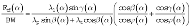
Figure 8.10 Mechanical model of squat with horizontally moving center of gravity.
while the ϕ(α)‐function is described as [27]

The parameters of the equation are summarized in Table 8.4.
Table 8.4 Parameters of the tibiofemoral force and ϕ function [27].
| Parameter | Quantity or function | SD |
| λ1(α) | 0.0024·α + 0.492 (–) | 0.15 |
| β(α) | −0.3861·α + 26.56 (°) | 14 |
| ø(α)(ø = γ/α) | −0.0026·α + 0.567 (–) | 0.081 |
| λt | 0.11 (–) | 0.018 |
| λp | 0.1475 (–) | 0.043 |
If Equation (8.7) is multiplied by an arbitrarily chosen BW then the tibiofemoral force is obtained. In the abovementioned analytical expressions, λ1 function describes the horizontal movement of the center of gravity during squat. If the linear function is used as given in Table 8.4, then a more realistic, so‐called non‐standard squat is carried out where the torso leans forward, and it helps the knee to release a considerable amount of moment (Figure 8.11). This is the squat type that is practiced by most people in everyday life.

Figure 8.11 Standard (non‐moving CoG) and non‐standard (moving CoG) squatting.
The so‐called standard squat is defined for tests and simple mechanical modeling. Nonetheless, it does not consider the movement of the torso during the motion; therefore, higher knee moment, tibio‐ and patellofemoral forces act in the knee if this motion is considered. With this model, both motions, and therefore the two types of tibiofemoral forces, are analyzed with their impact on wear.
When the non‐standard squat is being examined the λ1 function is constant with a value of 1. This means that the torso does not lean forward (Figure 8.11, left drawing). In case the non‐standard squat is exercised, the torso leans forward, which is modeled by a flexion angle dependent λ1(α) function (Figure 8.11, right drawing).
In the augmented wear equation, the tibiofemoral force will be included as follows:
If the tibiofemoral force is indexed as Ftf−nst CoG then the horizontal movement of the center of gravity is also included, while with the index of Ftf−st CoG, the forward lean of the torso, the horizontal motion of the center of gravity, is excluded.
8.3.3 Slide–Roll Modeling for Wear Equation
Slide–roll is known to be an important parameter of wear; however, its quantitative effect has not been studied earlier. By knowing the slide–roll function, exact conclusions can be drawn about the features of the motion. If the ratio is 0 then pure rolling is present, while 1 describes pure sliding. If the ratio is between 0 and 1, the movement is characterized as partial rolling and sliding. For example, a sliding–rolling ratio of 0.4 means 40% of sliding and 60% of rolling. Fekete et al. [20] introduced the slide–roll ratio by having the arc lengths on both connecting bodies as follows:

where
are the corresponding incremental differences of the connecting arc lengths.
A positive ratio shows the slip of the femur compared to the tibia. By this definition, the author derived an averaged slide–roll ratio with a standard deviation (SD = 0.136) based on several TKRs as a function of flexion angle [20]:
This function is used further on in the calculations, and it is assumed that the function is applicable for flexion and extension movement as well. With respect to the slide–roll ratio, there is an accordance between the authors that sliding is not dominant up to 65–67° of flexion angle [17, 18], which practically represents the domain of gait swing.
Nägerl et al. [19] and Fekete et al. [20] derived lower ratios between 0 and 65–67 flexion angle (Figure 8.12), and above this region they presume that the slide–roll ratio can reach 95% of sliding as well [19]. The interpretation for why these ratios have such discrepancies is likely to be credited to the simplifications, e.g. frictionless contact, two‐dimensional, simple circle or simplified knee geometry that the earlier authors applied in their models [17, 18]. Nägerl et al. [19] used the first‐time three‐dimensional geometry to derive the slide–roll ratio, while Fekete et al. [20] included the effect of friction besides three dimensionality in their three‐dimensional models.

Figure 8.12 Summarized slide–roll ratios from different authors.
Owing to these enhancements, the latter two authors revealed a nonlinear phenomenon in the trend of the slide–roll ratio. Since slide–roll is known, it must be involved in the wear calculation to quantify its effect. To include the slide–roll ratio into the equation, let us rewrite the length of sliding as the product of sliding velocity (m s−1) and infinitesimal time (s).
The definition of slide–roll according to Fekete et al. [20] can be expressed by the tangential velocities instead of the arc lengths:

where vCTt and vCFt are the tangential velocities in the instantaneous contact points. The difference between these velocities (vCTt − vCFt = vsliding) provides the so‐called sliding velocity. If Equation (8.13) is rearranged to vsliding then it can be included in our equation and we obtain the augmented Archard’s law:
vCTt velocity is kept constant similar to a wear test parameter [10] as an approximation. The original function of Ftf is the function of flexion angle [20], but it can be transformed into time domain. This has been carried out from the study of Fekete et al. [20], where the data were obtained also in time domain during the squat simulation. Thus, the final equation is as follows:
The parameters for the equation are summarized in Table 8.5.
Table 8.5 Wear parameters.
| Parameter | Quantity or function |
| k: Specific wear rate [10] | 1.3 × 10⁻⁶ (mm3 N−1 m−1) |
| μk: Coefficient of kinetic friction [20] | 0.003 (–) |
| Ftf/BW: Tibiofemoral force relative to the body weight (moving CoG) | 0.770 2·t3 + 0.554·t2 + 1.624 4·t + 1.031 1 (–) |
| Ftf/BW: Tibiofemoral force relative to the body weight (non‐moving CoG) | 0.665 2·t3 + 0.439 7·t2 + 3.262·t + 1.056 4 (–) |
| S/R: varying slide–roll ratio | −0.111 667·t3 + 0.363 173 2·t2 + 0.023 783 65·t + 1.137 558 (–) |
| S/R: constant slide–roll ratio | 0.4 (–) |
| BW: body weight | 1000 (N) |
| vCTt: Tangential velocity of the tibia in the contact | 30 (mm s−1) |
| t: Duration of motion | During squat: 1.53 (s) |
In the following, six total wear volumes will be calculated, each of them during one squat cycle. One cycle in squat is defined between 0° and 120° of flexion while the complete range where the propagation of wear monitored is 15 years. A usual knee wear simulation period is 3.5 million cycles [30, 31]; however, squat and deep squat are less frequently exercised in everyday life.
If 3.5 million cycles were broken down over 15 years, it would mean 640 complete deep squat cycles carried out daily. This number of cycles is clearly overestimated; thus 50 deep squats per day will be assumed in this chapter. The total wear during one cycle can be calculated by integrating the wear functions over time. During deep squat, the total cycle will be expanded to 120° of flexion angle where the time interval goes from 0 to 3.06 s during the squat motion (Figure 8.13).

Figure 8.13 Wear propagation of the different models.
The total wear volumes are calculated in the following way: firstly, the slide–roll ratio is kept constant with the number 0.4 according to the study of McGloughlin and Kavanagh [17] together with Hollmann et al. [18] while a standard squat is carried out (the tibiofemoral force does not have the effect of the horizontally moving center of gravity). Secondly, the slide–roll ratio varies according to the function of Fekete et al. [20] while a standard squat is carried out as well. Thirdly, the slide–roll ratio is kept constant with the number 0.4, but non‐standard squat is considered (horizontally moving center of gravity), while fourthly, the slide–roll ratio varies during the non‐standard squat.
In the last two calculations, similarly to a wear test on a pin‐on‐disk or ball‐on‐disk configuration, the slide–roll ratio is kept constant at 0.4 in one case, while in the other case it varies.
Regarding the force, only the simple Coulomb law (Fs = μk FN) is considered, which results in a constant load. The general method to calculate total wear during one squat cycle is as follows:


In the first calculations, both models use the tibiofemoral force where the horizontal movement of the center of gravity is included (non‐standard squat “nst”). Thus, the total wear with varying slide–roll ratio is
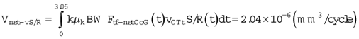
while the total wear with constant slide–roll ratio is

In the second calculation, both models use the tibiofemoral force where the center of gravity does not move horizontally (standard squat “st”).
- Total wear with varying slide–roll ratio but without the horizontal movement of the center of gravity:

- Total wear with constant slide–roll ratio:

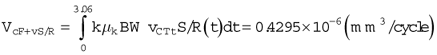
- Total wear if constant load (BW) and constant slide–roll ratio are used:

- And, at last, total wear if constant load (BW) and variable slide–roll ratio are used:
8.4 Results
The calculations of the integrals have been summarized in Table 8.6, where the percentile difference of the new parameters can be observed. By looking at the calculation of the wear test condition, only 1% difference is observable when varying or constant slide–roll ratio is applied. Therefore, the number of 0.429 × 10⁻⁶ (mm3/cycle) can be chosen as a point of reference.
Table 8.6 Wear results and comparison.
| Standard squat | Non‐standard squat | ||||
| Wear volume (10−6 mm3/cycle) |  |  |  |  | |
| Wear test condition | Vc F + c S/R = 0.4289 | 5.5 | 6.25 | 4.16 | 4.75 |
| Vc F + v S/R = 0.4295 | |||||
| Standard squat | Vst − v S/R = 2.68 | ||||
| Vst − c S/R = 2.33 | |||||
| Non‐standard squat | Vnst − v S/R = 2.04 | ||||
| Vnst − c S/R = 1.76 | |||||
When the results from the standard and non‐standard squat are compared to the reference value, it is visible that the wear, generated by the augmented models, is assumed to be 4.16–6.25 times more compared to the reference value.
The significant difference is due to the new parameters, the varying tibiofemoral force function, and the slide–roll ratio. As for quantitative conclusions, the total wear with constant slide–roll ratio during standard squat (Vconst S/R) is expected to be 5.5 times higher compared to the reference value (VW test), while if total wear includes varying slide–roll ratio during standard squat, then the calculated wear is ~6.25 times higher.
With regard to non‐standard squat, total wear with constant slide–roll ratio during standard squat (Vconst S/R) is expected to be 4.16 times higher compared to the reference value (VW test), while if the total wear includes varying slide–roll, then the calculated wear is ~4.75 times higher.
In case the wear model is coupled with constant slide–roll ratio under non‐standard squatting as compared to a wear model where the slide–roll ratio varies and standard squat is considered, then a 65% higher wear volume can be expected with respect to the model with standard squat movement.
It is easy to notice that the highest wear volume is generated in the case of standard squat due to the fact that the tibiofemoral force, without the effect of the horizontal lean of the torso, will reach the highest magnitude compared to other squatting motion. This makes the tibiofemoral force probably the most dominant parameter in the augmented Archard’s law.
According to Figure 8.13, the varying slide–roll ratio has also the effect of increasing the wear volume. A feasible explanation for why the wear volume is lower when constant 0.4 (40% of sliding) slide–roll ratio is considered during squat can be addressed as follows: it has been proved by several studies that during flexion of the knee joint, approximately up to 20–30° of flexion, rolling is dominant [19, 20], which is not a crucial motion as far as wear is concerned, since the friction effect caused by sliding is also very low.
Therefore, the authors who considered 0.3–0.4 slide–roll ratio were correct with respect to the beginning of the motion of squat, but not with respect to the complete cycle. Above 30° of flexion, as sliding prevails, wear starts developing between the surfaces due to shear stress, which is caused by the increasing slide [30]. Since the kinematic condition of the TKR geometries is different, wear must differ during the progression of the motion as well, which can be observed in Figure 8.13.
The propagation of wear for the lifetime cycle has been calculated as well, as seen in Figure 8.14.

Figure 8.14 Total wear during lifetime cycle.
Evidently, in case the wear test model is considered, where the load is constant different slide–roll ratio types (constant or varying) have negligible effect on wear in the long term.
8.5 Discussion
The effect of the new parameters on wear, the slide–roll ratio, and the tibiofemoral force with and without the horizontal movement of the center of gravity have been evidently demonstrated and quantitatively determined. Varying slide–roll ratio as a wear parameter causes approximately 15% more wear than constant slide–roll ratio, regarding any type of squatting motion. The involvement of the tibiofemoral force has a major effect on wear, which can lead to 65% more removed volume per cycle compared to other configurations.
As a further step, on one hand, the augmented wear model is to be applied for other types of movements, such as gait or even specific motions, e.g. cutting movement in football. This can be carried out by knowing the load case (load function) during these motions. On the other hand, if the specific wear coefficients of NFCs could be estimated with higher load cases as well, then the model would be appropriate to estimate wear propagation in the case where these materials played a role in a TKR configuration instead of a standard UMHWPE material.
Limitations of the study must be pointed out as well. The friction force is calculated by the simple Coulomb law, which assumes a point connection, while in reality the contact is a surface. The specific wear rate (k) can highly alter the phenomenon, and it can be only obtained via experiments for different kinematic conditions coupled with diverse materials. It should be studied further how well it is possible to estimate the correct k value from the literature in order to gain adequate results for the mathematical analysis.
Acknowledgments
This work was supported by the ELTE Eötvös Loránd University in the frame of the ÚNKP‐17‐4 New National Excellence Program of the Ministry of Human Capacities, the National Natural Science Foundation of China (81301600) and Anta Sports Products Limited (HK2015000090), the Savaria Institute of Technology, and the Research Academy of Grand Health, Ningbo University.
References
- 1 Ashby, M.F. (2009). Material Selection in Mechanical Design. Elsevier.
- 2 Young, R.J. (2011). Introduction to Polymers, 3e. Taylor & Francis Group.
- 3 Rao, K.M.M. and Rao, K.M. (2007). Extraction and tensile properties of natural fibers: Vakka, date and bamboo. Composite Structures 77: 288–295.
- 4 Bhushan, B. (2001). Modern Tribology Handbook. CRC Press.
- 5 Sharkey, P.F., Lichstein, P.M., Shen, C. et al. (2014). Why are total knee arthroplasties failing today – has anything changed after 10 years? Journal of Arthroplasty 29: 1774–1778.
- 6 Chittaranjan, D. and Acharya, S.K. (2010). Effects on fiber content on abrasive wear of Lantana camara fiber reinforced polymer matrix composite. Indian Journal of Engineering and Material Sciences 17: 219–223.
- 7 Ren, G., Zhang, Z., Song, Y. et al. (2017). Effect of MWCNTs‐GO hybrids on tribological performance of hybrid PTFE/Nomex fabric/phenolic composite. Composite Science and Technology 146: 155–160.
- 8 Omrani, E., Menezes, P.L., and Rohatgi, P.K. (2016). State of the art on tribological behavior of polymer matrix composites reinforced with natural fibers in the green materials world. Engineering Science and Technology, an International Journal 19 (2): 717–736.
- 9 Yousif, B.F. and El‐Tayeb, N.S.M. (2009). Wet adhesive wear characteristics of untreated oil palm fibre‐reinforced polyester and treated oil palm fibre‐reinforced polyester composites using the pin‐on‐disc and lock‐on‐ring techniques. Proceedings of the Institution of Mechanical Engineers, Part J: Journal of Engineering Tribology 224: 123–131.
- 10 Patten, E.W., Van Citters, D., Ries, M.D., and Pruitt, L.A. (2013). Wear of UHMWPE from sliding, rolling, and rotation in a multidirectional tribo‐system. Wear 304 (1–2): 60–66.
- 11 Karlhuber, M. (1995) Development of a method for the analysis of the wear of retrieved polyethylene components of total knee arthroplasty. Thesis. Technical University of Hamburg, Germany.
- 12 Guo, Y., Hao, Z., and Wan, C. (2016). Tribological characteristics of polyvinylpyrrolidone (PVP) as a lubrication additive for artificial knee joint. Tribology International 77: 214–219.
- 13 Qiu, M., Chyr, A., Sanders, A.P., and Raeymaekers, B. (2014). Designing prosthetic knee joints with bio‐inspired bearing surfaces. Tribology International 77: 106–110.
- 14 Wimmer, M.A. and Andriacchi, T.P. (1997). Tractive forces during rolling motion of the knee: implications for wear in total knee replacement. Journal of Biomechanics 30 (2): 131–137.
- 15 Lopez‐Cervantes, A., Dominguez‐Lopez, I., Barceinas‐Sanchez, J.D.O., and Garcia‐Garcia, A.L. (2013). Effects of surface texturing on the performance of biocompatible UHMWPE as a bearing material during in vitro lubricated sliding/rolling motion. Journal of the Mechanical Behavior of Biomedical Materials 20: 45–53.
- 16 Rawal, B.R., Yadav, A., and Pare, V. (2016). Life estimation of knee joint prosthesis by combined effect of fatigue and wear. Procedia Technology 23: 60–67.
- 17 McGloughlin, T. and Kavanagh, A. (1998). The influence of slip ratios in contemporary TKR on the wear of ultra‐high molecular weight polyethylene (UHMWPE): an experimental view. Journal of Biomechanics 31: 8.
- 18 Hollman, J.H., Deusinger, R.H., Van Dillen, L.R., and Matava, M.J. (2002). Knee joint movements in subjects without knee pathology and subjects with injured anterior cruciate ligaments. Physical Therapy 82: 960–972.
- 19 Nägerl, H., Frosch, K.H., Wachowski, M.M. et al. (2008). A novel total knee replacement by rolling articulating surfaces. In vivo functional measurements and tests. Acta of Bioengineering and Biomechanics 10 (1): 55–60.
- 20 Fekete, G., De Baets, P., Wahab, M.A. et al. (2012). Sliding–rolling ratio during deep squat with regard to different knee prostheses. Acta Polytechnica Hungarica 9 (5): 5–24.
- 21 Laurent, M.P.T., Johnson, S., Yao, J.Q. et al. (2003). In vitro lateral versus medial wear of knee prosthesis. Wear 255 (7–12): 1101–1106.
- 22 Archard, J.F. and Hirst, W. (1956). The wear of metals under unlubricated conditions. Proceedings of the Royal Society A 236: 397–410.
- 23 Pal, S., Haider, H., Laz, P.J. et al. (2008). Probabilistic computational modeling of total knee replacement wear. Wear 264 (7–8): 701–707.
- 24 O’Brien, S.T., Bohm, E.R., Petrak, M.J. et al. (2014). An energy dissipation and cross shear time dependent computational wear model for the analysis of polyethylene wear in total knee replacements. Journal of Biomechanics 47 (5): 1127–1133.
- 25 Turell, M., Wang, A., and Bellare, A. (2003). Quantification of the effect of cross‐path motion on the wear rate of ultra‐high molecular weight polyethylene. Wear 255 (7–12): 1034–1039.
- 26 Abdelgaied, A., Liu, F., Brockett, C. et al. (2011). Computational wear prediction of artificial knee joints based on a new wear law and formulation. Journal of Biomechanics 44 (6): 1108–1116.
- 27 Fekete, G., Csizmadia, B.M., Wahab, M.A. et al. (2014). Patellofemoral model of the knee joint under non‐standard squatting. Dyna Colombia 81 (183): 60–67.
- 28 Slater, L.V. and Hart, J.M. (2017). Muscle activation patterns during different squat techniques. Journal of Strength and Conditioning Research 31 (3): 667–676.
- 29 Slater, L.V. and Hart, J.M. (2016). The influence of knee alignment on lower extremity kinetics during squats. Journal of Electromyography and Kinesiology 31: 96–103.
- 30 Liu, A., Jennings, L.M., Ingham, E., and Fisher, J. (2015). Tribology study of natural knee using and animal model in a new whole joint natural knee simulator. Journal of Biomechanics 48 (12): 3004–3011.
- 31 Brockett, C.L., Carbone, S., Fisher, J., and Jennings, L.M. (2017). PEEK and CFR‐PEEK as alternative bearing materials to UHMWPE in a fixed bearing total knee replacement: an experimental wear study. Wear 374–375: 86–91.