Chapter 1
Synthetic Vision Using Volume Learning and Visual DNA
Whence arises all that order and beauty we see in the world?
―Isaac Newton
Overview
Imagine a synthetic vision model, with a large photographic memory, that learns all the separate features in each image it has ever seen, which can recall features on demand and search for similarities and differences, and learn continually. Imagine all the possible applications, which can grow and learn over time, only limited by available storage and compute power. This book describes such a model.
This is a technical and visionary book, not a how-to book, describing a working synthetic vision model of the human visual system, based on the best neuroscience research, combined with artificial intelligence (AI), deep learning, and computer vision methods. References to the literature are cited throughout the book, allowing the reader to dig deeper into key topics. As a technical book, math concepts, equations, and some code snippets are liberally inserted describing key algorithms and architecture.
In a nutshell, the synthetic vision model divides each image scene into logical parts similar to multidimensional puzzle pieces, and each part is described by about 16,000 different Visual DNA metrics (VDNA) within a volume feature space. VDNA are associated into strands—like visual DNA genes—to represent higher-level objects. Everything is stored in the photographic visual memory, nothing is lost. A growing set of learning agents continually retrain on new and old VDNA to increase visual knowledge.
The current model is a first step, still growing and learning. Test results are included, showing the potential of the synthetic vision model. This book does not make any claims for fitness for a particular purpose. Rather, it points to a future when synthetic vision is a commodity, together with synthetic eyes, ears, and other intelligent life.
You will be challenged to wonder how the human visual system works and perhaps find ways to criticize and improve the model presented in this book. That’s all good, since this book is intended as a starting point—to propose a visual genome project to allow for collaborative research to move the synthetic model forward. The visual genome project proposed herein allows for open source code development and joint research, as well as commercial development spin-offs, similar to the Human Genome Project funded by the US government, which motivates this work. The visual genome project will catalog Visual DNA on a massive scale, encouraging collaborative research and commercial application development for sponsors and partners.
Be prepared to learn new terminology and concepts, since this book breaks new ground in the area of computer vision and visual learning. New terminology is introduced as needed to describe the concepts of the synthetic vision model. Here are some of the key new terms and concepts herein:
–Synthetic vision: A complete model of the human visual system; not just image processing, deep learning, or computer vision, but rather a complete model of the visual pathway and learning centers (see Figure 1.1). In the 1960s, aerospace and defense companies developed advanced cockpit control systems described as synthetic vision systems, including flight controls, target tracking, fire controls, and flight automation. But, this work is not directed toward aerospace or defense (but could be applied there); rather, we focus on modeling the human visual pathway.
–Volume learning: No single visual feature is a panacea for all applications, so we use a multivariate, multidimensional feature volume, not just a deep hierarchy of monovariate features as in DNN (Deep Neural Networks) gradient weights. The synthetic model currently uses over 16,000 different types of features. For example, a DNN uses monovariate feature weights representing edge gradients, built up using 3×3 or n×n kernels from a training set of images. Other computer vision methods use trained feature descriptors such as the scale-invariant feature transform (SIFT), or basis functions such as Fourier features and Haar wavelets.
–Visual DNA: We use human DNA strands as the model and inspiration to organize visual features into higher-level objects. Human DNA is composed of four bases: (A) Adenine, (T) Thymine, (G) Guanine, and (C) Cytosine, combined in a single strand, divided into genes containing related DNA bases. Likewise, we represent the volume of multivariate features as strands of visual DNA (VDNA) across several bases, such as (C) Color, (T) Texture, (S) Shape, and (G) Glyphs, including icons, motifs, and other small complex local features.
Many other concepts and terminology are introduced throughout this work, as we break new ground and push the boundaries of visual system modeling. So enjoy the journey through this book, take time to wonder how the human visual system works, and hopefully add value to your expertise along the way.

Synthetic Visual Pathway Model
The synthetic vision model, shown in Figure 1.1, includes a biologically plausible Eye/LGN Model for early vision processing and image assembly as discussed in Chapter 2, a Memory Model that includes several regional processing centers with local memory for specific types of features and objects discussed in Chapter 4, and a Learning/Reasoning Model composed of agents that learn and reason as discussed in Chapter 4. Synthetic Neural Clusters are discussed in Chapter 6, to represent a group of low-level edges describing objects in multiple color spaces and metric spaces, following the standard Hubel and Weisel theories [1] that inspired DNNs. The neural clusters allow low-level synthetic neural concepts to be compared. See Figures 1.2, 1.3, and 1.4 as we go.
In this chapter, we provide several overview sections describing the current synthetic visual pathway model, with model section details following in subsequent Chapters 2–11. The resulting volume of features and visual learning agents residing within the synthetic model are referred to as the visual genome model (VGM). Furthermore, we propose and discuss a visual genome project enabled by the VGM to form a common basis for collaborative research to move synthetic vision science forward and enable new applications, as well as spin off new commercial products, discussed in Chapter 12.
We note that the visual genome model and corresponding project described herein is unrelated to the work of Krishna et al. [163][164] who use crowd-source volunteers to create a large multilabeled training set of annotated image features, which they call a visual genome.
Some computer vision practitioners may compare the VGM discussed in this book to earlier research such as parts models or bag-of-feature models [1]; however the VGM is out of necessity much richer in order to emulate the visual pathway. The fundamental concepts of the VGM are based on the background research in the author’s prior book, Computer Vision Metrics: Survey, Taxonomy, and Analysis of Computer Vision, Visual Neuroscience, and Deep Learning, Textbook Edition (Springer-Verlag, 2016), which includes nearly 900 references into the literature. The reader is urged to have a copy on hand.
Visual Genome Model
The VGM is shown in Figure 1.2 and Figure 1.4; it consists of a hierarchy of multivariate feature types (Magno, Parvo, Strands, Bundles) and is much more holistic than existing feature models in the literature (see the survey in [1]). The microlevel features are referred to as visual DNA or VDNA. Each VDNA is a feature metric, described in Chapters 4–10. At the bottom level is the eye and LGN model, described in Chapters 2 and 3. At the top level is the learned intelligence—agents—as discussed in Chapter 4. Each agent is a proxy for a specific type of learned intelligence, and the number of agents is not limited, unlike most computer vision systems which rely on a single trained classifier. Agents evaluate the visual features during training, learning, and reasoning. Agents can cooperate and learn continually, as described in Chapter 4.
Visual genomes are composed together from the lower level VDNA features into sequences (i.e. VDNA strands and bundles of strands), similar to a visual DNA chain, to represent higher-level concepts. Note that as shown in Figure 1.2, some of the features (discussed in Chapter 6) are stored as content-addressable memory (CAM) as neural clusters residing in an associative memory space, allowing for a wide range of feature associations. The feature model including the LGN magno and parvo features is discussed in detail in Chapters 2, 3, and 4.
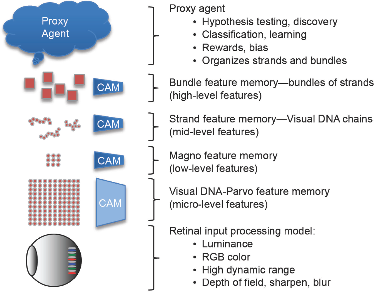
The VGM follows the neurobiological concepts of local receptive fields and a hierarchy of features, similar to the Hubel and Wiesel model [146][147] using simple cells and complex cells. As shown in Figure 1.2, the hierarchy consists of microlevel VDNA parvo features which are detailed and high resolution, low resolution magno features, midlevel strands of features, and high-level bundles of strands as discussed below. Each feature is simply a metric computed from the memory record of the visual inputs stored in groups of neuron memory. This is in contrast to the notion of designing a feature descriptor to represent a group of pixels in a compressed or alternative metric space as done in traditional computer vision methods.
VGM stores low-level parvo and magno features as raw memory records or pixel impressions and groups the low-level VDNA memory records as strands and groups of strands, which are associated together as bundles describing higher-level concepts. For texture-like emulation of Hubel and Weisel neuron cells, the raw input pixel values of local receptive fields are used to compose a feature address vector referencing a huge virtual multidimensional address space (for more details see Chapter 6, Figures 6.1, 6.2, 6.3). For CAM features, the address is the feature. The intent of using the raw pixel values concatenated into a CAM address is to enable storage of the raw visual impressions directly in a virtually unlimited feature memory with no intervening processing, following the view-based model of neurobiology. The bit precision of the address determines the size of the memory space. The bit precision and coarseness of the address is controlled by a quantization parameter, discussed later along with the VGM neural model. So, the VGM operates in a quantization space, revealing more or less detail about the features as per the quantization level in view.
Volume Learning
The idea of volume learning is to collect, or learn, a large volume of different features and metrics within a multivariate space, including color, shape, texture, and conceptual glyphs, rather than collecting only a nonvolumetric 1D list of SIFT descriptors, or a hierarchical (i.e. deep) set of monolithic gradient features such as DNN convolutional weight templates. Volume learning implies a multidimensional, multivariate metric space with a wide range of feature types and feature metrics, modeled as VDNA. We suggest and discuss a robust baseline of VDNA feature metrics in great detail in Chapters 5–10, with examples tested in Chapter 11. Of course, over time more feature metrics will be devised beyond the baseline.
Proxy agents, discussed in detail in Chapter 4, are designed to learn and reason based on the volume of features. So, many styles of learning and reasoning are enabled by volume learning.
In fact, agents can model some parts of human consciousness which seem to be outside of the neurobiology itself. Such higher-level consciousness, as emulated in agents, can direct the brain to explore or learn based on specific goals and hypotheses. In this respect, the VGM provides a synthetic biological model of a brain enabling proxy agents with varying IQs and training to examine the same visual impressions and reach their own conclusions. Each proxy agent encodes learnings and values similar to recipes, algorithms, priorities, likes, dislikes, and other heuristics. Proxy agents exist in the higher-level PFC regions of the brain, along with strands, bundles, and other higher-level structures specific to each proxy agent. Thus, domain-specific or application learning is supported in the VGM, built on top of the visual impressions in the VGM.
Volume learning is also concerned with collecting a large volume of genomes and features over time—continuous learning. So, volume learning is analogous to the Human Genome Project: sequence first, label and classify later. It is expected that billions of images can be sequenced to identify the common visual genomes and VDNA; at that point, labeling and understanding can begin in earnest. Even prior to reaching saturation of all known visual genomes (if possible), classification and labeling can occur on a grand scale. Figure 1.3 illustrates the general process of learning new genomes from new visual impressions over time: as the number of impressions in memory grows, the number of unique new features encountered decreases. That is where the visual genome project gets interesting.

Volume learning and the VGM assumes that the sheer number of features is more critical than the types of features chosen, as evidenced by the feature learning architecture survey in [1] Chapters 6 and 10, which discusses several example systems that achieve similar accuracy based on a high number of features using differing feature types and feature hierarchies. It is not clear from convolutional neural networks (CNNs) research that the deep hierarchy itself is the major key to success. For example, large numbers of simple image pixel rectangles have been demonstrated by Gu et al. [148] to be very capable image descriptors for segmentation, detection, and classification. Gu organizes the architecture as a robust bag of overlapped features, using Hough voting to identify hypothesis object locations, followed by a classifier, to achieve state-of-the-art accuracy on several tests. The VGM follows the intuition that the sheer number of features is valuable and offers over 16,000 feature dimensions per genome and over 56,000 feature comparison metrics per each reference/target genome comparison, using various distance functions as discussed in Chapters 2–10.
Classifier Learning and Autolearning Hulls
Classifier learning is a novel method developed in the VGM, and allows several independent classifiers to be learned in separate agents from the large volume of VDNA features. Classifier learning takes place after the volume feature learning, based on a chosen training protocol used by an agent. Several agents may take a different training protocol and then the agents may operate together in an ensemble. VGM supports complex, structured classifiers as discussed in Chapter 4.
Many traditional vision systems rely on a simple final classifier stage, such as a SOFTMAX or support vector machine (SVM), to perform matching and inference [1]. However some classifier models, such as the Inception DNNs [158], use a branching DNN structure with classifiers scattered at branch terminus. However, the common element in typical DNN classifiers is that the classifier acts on a set of learned feature weights, but the classifier is not learned: the classifier method used is a design decision, and the classifier is manually tuned to operate on accumulated feature match thresholds during testing. As discussed in [1], Feed Forward (FF) DNNs develop a hierarchical model consisting of a 1D vector of uncorrelated monovariate weights (for example, double precision numbers or weights), but VDNA metrics enable a volume learning model consisting of a multivariate feature set. A volume of individual metrics is expressive, allowing for a richer classifier.
Autolearning hulls are a form of metric learning discussed in detail in Chapter 4. Each autolearning hull provides a biologically plausible feature match hull threshold for each metric to assist in building up structured multivariate classifiers from sets of metrics. First, as discussed in Chapters 2 and 3, each feature metric is computed within the various biological eye/LGN model spaces raw, sharp, retinex, histeq, and blur. Currently, this yields ~16,000 independent feature metrics per genome region. Next, a hull representing the biologically plausible variance of each of the ~16,000 feature metrics within the eye/LGN spaces is computed. During learning, the hulls are sorted to find the metrics with the tightest hull variation to use as a first-order set of metrics to be further tuned via a form of agent-based reinforcement learning to optimize the metric hulls to achieve the best correspondence with the training set. See Chapter 4.
The VGM model allows for classifiers to be learned and implemented in separate agents, similar to the way humans manage a specific knowledge domain using domain-specific contextual rules, allowing each agent to define the learning and reasoning domain for a given task, rather than relying on a single classifier. Therefore, the autolearning method establishes a biologically plausible first-order default hull range around each feature metric for correspondence and matching. The default first-order hulls are used by an agent as a starting point to establish a first-order classifier, and then the first-order metrics are tuned via a variant of reinforcement learning and composed into an optimized classifier during training. Several classifiers may be learned by separate agents for each genome, based on various robustness criteria, training protocols, or other heuristics. See the discussions in Chapters 4 and 5.
Visual Genome Project
The visual genome project will be an open repository of visual knowledge to apply and leverage the visual genome model (VGM) within a common software infrastructure and platform, enabling a consortium of vision scientists and engineers to collaboratively move vision science forward by cataloging unique visual features, and visual learning agents, see Figure 1.4. The synthetic visual pathway model is informed by the research and survey into human vision, neuroscience, computer vision models, artificial intelligence, deep learning, and statistical analysis in the author’s text Computer Vision Metrics, Textbook Edition [1]. The synthetic visual pathway model includes plausible models of the biology and mechanisms of human vision. More background research is covered later in this chapter as well.
The synthetic visual pathway model concepts are developed in detail within Chapters 2–10. The learning agents model is developed in Chapter 4. In Chapter 11 we illustrate the models in a complete synthetic vision system test; to sequence visual genome features for a specific environment; train learning agents to find the specific visual genomes; and provide results, analysis, discussion. Chapter 12 points to future work and details on the visual genome project.
We take inspiration from the Human Genome Project and the Human Connectome Project, discussed later in this chapter, which demonstrate some of the best attributes of collaborative science projects. We expect synthetic vision to provide benefits analogous to other sciences such as prosthetics and robotics, where specific attributes of human biology and intelligence are analyzed, modeled, and deployed. Synthetic vision is another step along the trend in artificial biology and artificial intelligence.
The models described herein are considered to be among the most novel and comprehensive in the literature and form the basis and starting point for future work into better visual pathway models, allowing an entire ecosystem of open source agents to be built by developers on a standard visual genome platform, using a common set of VDNA.
Major goals of the visual genome project include:
–Common VDNA Catalog: One goal is to create a catalog and database of VDNA and sequences of VDNA, including strands, bundles, objects, and genes as described in Chapter 3 (for specific application domains, see Figure 1.4). Once a set of specific VDNA is catalogued in the database, the VDNA is used by agents for comparison, correspondence, associations, learning, and reasoning. In addition, catalogued VDNA can be assigned a unique VDNA_ID number, providing memory and communications bandwidth savings for some agent methods and applications. Large numbers of VDNA will be catalogued for specific application domains, enabling learning agents to leverage VDNA that are already known. Over time, the VDNA catalog can be made as large as possible, providing high-level advantages to vision science to develop a massive VDNA sequence, similar to the Human Genome Project. This is a realistic goal, given that the resolution of the data is sufficiently compact, and commodity data storage capacity is increasing.
–Common Learning Agents: Another goal is to create a repository of common set of learning agents trained for specific application domains. The visual genome format enables the learning agents to operate within a common feature space and metric space, allows for extensions, and enables the agents to work together and share agents in the repository.
–Common Application Programming Interface (API) and Open Developer Ecosystem: Both commercial use and collaborative research use of the synthetic vision model as an ecosystem can occur simultaneously, based on an open, standardized platform and API. Researchers can create and share a very large collection of visual genomes and agents for open access, while commercialized agents and VDNA can be developed as well. Effectively, the ecosystem is like the movie The Matrix, where knowledge and understanding (agents) can be deployed and downloaded for specific purposes.

As shown in Figure 1.4, the term CSTG refers to the multivariate VGM feature bases Color (C), Shape (S), Texture (T), and Glyph (G), discussed in detail in Chapter 3 (see especially Figure 3.6).
Master Sequence of Visual Genomes and VDNA
The end goal of the visual genome project is to sequence every image possible, create a master list of all the genomes and VDNA, and assign each genome a unique 16-byte sequence number initially in a 1 petabyte (PB) genome space. Once sequenced, each genome and associated metrics will be kept in a master database or VDNA catalog keyed by sequence numbers. It is envisioned that 1PB of unique genome IDs will be adequate for sequencing a massive set of visual images; assuming 3000 genome IDs per 12 megepixel image, 1PB of genome ID space is adequate for sequencing about 333 gigaimages. Images which contain genomes matching previously cataloged genomes can share the same genome IDs and storage space, so eventually finding common genomes will reducing storage requirements
Like the Human Genome Project, the end goal is a complete master sequence of all possible VDNA, which will reveal common genomes and accelerate image analysis and correlation. Storage capability challenging today’s largest file systems will be required. The Phase 1 visual genome project is estimating 3–5 petabytes of storage required to sequence 1 million images and store all the image data, the visual DNA catalog, and the learning agent catalog. Phase 1 will store comprehensive metrics for research purposes. Application specific VDNA catalogs will be space optimized, containing only application essential VDNA metrics, reduced to a small memory footprint to fit common computing devices.
VGM API and Open Source
The VGM API provides controls for the synthetic visual pathway model and is available as open source code with an API for local development, or as a cloud-based API for remote systems to leverage a complete VGM in the cloud. The API includes methods to create private genome spaces to analyze specific sets of images, as well as public genome spaces for collaborative work. The cloud-based API is a C++ library, rather than complete open source code. The entire C++ library code will be open sourced once the key concepts are developed and proven useful to the research community. Chapter 5 provides an overview of the VGM API. Chapter 12 provides open source details.
VDNA Application Stories
In this section, we provide background on some applications for the synthetic vision model, focusing on two key applications: (1) overcoming DNN spoofing by using DNN glyphs (i.e. trained weight models) in the VDNA model and (2) visual inspection and inventory for objects such as a car, a room, or a building by collecting genomes from the subject and detecting new or changed genomes to add to the subject VDNA set. We also suggest other applications for VDNA at the end of the section.
Overcoming DNN Spoofing with VGM
Current research into DNN models includes understanding why DNNs are easily spoofed and fooled in some cases (see Figure 1.5). We cover some of the background here from current DNN research to lay the foundation for using VDNA to prevent DNN spoofing. One problem with a basic DNN that enables spoofing is that each DNN model weight is disconnected and independent, with no spatial relationships encoded in the model. Also, there is limited invariance in the model, except for any invariance that can be represented in the training set. Invariance attributes are a key to overcoming spoofing (see [1]).
Part of the DNN spoofing problem relates to the simple monovariate features that are not spatially related, and the other part of the problem relates to the simple classifier that just looks for a critical mass of matching features to exceed a threshold. The VGM model overcomes these problems.
Note that the recently developed CapsNet [170] provides a method to overcome some invariance issues (and by coincidence eliminate some spoofing) by grouping neurons (e.g. feature weights) to represent a higher-level feature or capsule, using a concept referred to as inverse graphics to model groups of neurons as a feature with associated graphics transformation matrices such as scale and rotation. CapsNet currently is able to recognize 2D monochrome handwriting character features in the MNIST dataset at state-of-the-art levels. CapsNet does not address the most complex problems of 3D scene recognition, 3D transforms, or scene depth. However, well-known 3D reconstruction methods [1] have been successfully used with monocular, stereo, and other 3D cameras to make depth maps and identify objects in 3D scene space and create 3D graphics models (i.e. inverse graphics), as applied to real estate for mapping houses and rooms, as well as other applications. In any case, CapsNet is one attempt to add geometric invariance to DNNs, and we expect that related invariance methods for DNNs will follow- for example, an ensemble with two models: (1) the DNN weight model and (2) a corresponding spatial relationship model between DNN weights based on objects marked in the training data. CapsNet points to a future where we will see more DNN feature spatial relationships under various 2D and 3D transform spaces. The VGM can also be deployed with DNNs in an ensemble to add invariance to scene recognition as explained below. Gens and Domingos [99][1] describe a DNN similar to Capsnet, using deep symmetry networks to address the fundamental invariance limitations of DNNs, by projecting input patches into a 6-dimensional affine feature space.
Trained DNN models are often brittle and overtrained to the training set to such an extent that simple modifications to test images—even one-pixel modifications similar to noise—can cause the DNN inference to fail. DNNs are therefore susceptible to spoofing using specially prepared adversarial images. While DNNs sometimes work very well and even better than humans at some tasks, DNNs are also known to fail to inference correctly in catastrophic ways as discussed next.
Research into spoofing by Nguyen et al. [5] show the unexpected effects of DNN classification failure (see Figure 1.5). DNN failure modes are hard to predict: in some cases the images recognized by DNNs can look like noise (Figure 1.5 left) or like patterns (Figure 1.5 right) rather than the natural images they are trained on. Nguyen’s work uses DNNs trained on ImageNet data and MNIST data and then generates perturbed images using a gradient descent-based image generation algorithm which misleads the trained DNNs to mislabel with high confidence.

Some researchers believe that generating adversarial images using generative adversarial networks, or GANs, to test and prod other DNN models (see Goodfellow et al. [10]) has opened up a door to a new type of generative intelligence or unsupervised learning, with the goal of little to no human intervention required for DNN-based learning. Generative intelligence is a form of reinforcement learning, at the forefront current DNN research, where a DNN can generate a new DNN model by itself that refines its own model according to reinforcement or feedback criteria from another DNN. In other words, a DNN makes a new and better DNN all by itself by trying to fool another DNN. Generative intelligence will allow a student DNN to create models independently by studying a target DNN to (1) learn to emulate the target DNN, (2) learn to fool the target DNN, and then (3) learn to improve a new model of the target DNN. Generative adversarial networks (GANs) can be used to analyze training sets or reduce the size of the training set, as well as produce adversarial images to fool a DNN.
Visual genomes can be used to add a protective layer to an existing DNN to harden the classifier against spoofing, in part by using VDNA strands of features with spatial information including local coordinates and angles as discussed in Chapter 8. The visual genome platform solution to DNN spoofing is possible since the VDNA model incorporates VDNA, such as shape (S) and feature metric spatial relationships, color (C), texture (T), and glyph (G) features together, as well as complex agent classifiers. Therefore, the final classification does not depend solely on thresholding feature correspondence from the simple spatially unaware DNN model weights but rather incorporates a complete VDNA model designed tolerant to various robustness criteria.
To overcome DNN spoofing using VDNA, a DNN can be used together with the VGM model by associating VDNA with overlapping DNN features—overlaying a spatial dimension to the DNN model. Since DNN correspondence can be visualized spatially (see Zeiler and Fergus [11]) by both rendering the DNN weight matrices as images and also by locating the best corresponding pixel matrices in the corresponding image and highlighting the locations in the image, the genome region VDNA can be evaluated together with the DNN model score, providing additional levels of correspondence checking beyond the DNN weights (see Figure 1.6).
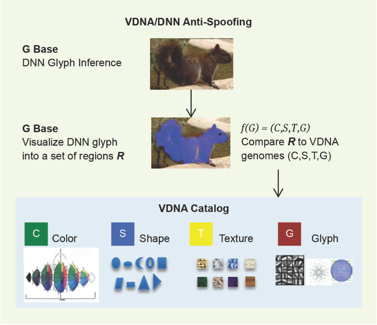
DNNs often produce glyph-like, realistic looking icons of image parts, resembling dithered average feature icons of parts of the training images (see [1], Figure 9.2), like learned correlation templates. While these glyphs are proven to be effective in DNN inference, there are also extreme limitations and failures, attributable to the primitive nature of correlation templates, as discussed in [1]. Also, the gradient-based training nature of DNNs favor gradients of individual weights of pixels, not gradients of solid regions of color or even texture. Furthermore, the DNN correlation templates are not spatially aware of each other, which is a severe DNN model limitation. Visual genomes overcome the limitations of DNN by providing a rich set of VDNA shape (S), color (C), texture (T), and glyph (G) bases, as well as spatial relationships between features supported in the VDNA model as illustrated in Figure 3.1. Using DNNs and the VGM together as an ensemble can increase DNN accuracy.
DNN failures and spoofing have been overcome by a few methods cited here; for example, using voting ensembles of similarly trained DNNs to weed out false inferences as covered by Bajuja, Covell, and Suthankar [3]. Also Wan [4] trains a hybrid DNN model + structured parts model together as an ensemble. The visual genome method includes hybrid feature models and is therefore similar to Wan’s method but uses a richer feature space with over 16,000 base features.
While many methods exist to perturb images to fool a DNN, one method studied by Baluja and Fischer [15] uses specially prepared gradient patterns taken from a trained DNN model combined with a test image. From a human perspective, the adversarial images may be easily recognized, but a DNN model may not have been trained to recognize such images. As shown in the paper, an image of a dog is combined with gradient information from a soccer ball, resulting in the DNN model recognizing the image as a soccer ball instead of a dog. Note that specific adversarial images may fool a specific trained DNN model, but will not necessarily fool other trained DNN models. Quite a bit of research is in progress to understand the spoofing phenomenon.
In many cases, adversarial images generated by a computer are not realistic and may never be found in natural images, so the adversarial threat can be dismissed as unlikely in some applications. However, Juraki et al. [19] show that adversarial images generated by computer and then printed onto paper and viewed on a mobile phone are effective in spoofing DNNs. While this work on adversarial images may seem academic, the results demonstrate how easily a malicious actor can develop adversarial images to spoof traffic signs, print them out, and place them over the real traffic signs to fool DNNs.
Another related DNN spoofing method to alter traffic signs is described and tested by Evtimov et al. [76] where certain patterns and symbols can be placed on a traffic sign, similar to decals, and the DNN can be spoofed 100% of the time according to their tests. In fact, just adding a Post-it sticker to a traffic sign is enough to fool the best DNN, as demonstrated in the Badnets paper [107] by Garg et al. (see also Evtimov et al. [107]). Clearly, DNNs are susceptible to spoofing, like other computer vision methods.
Papernot et al. [6] implement a method of generating adversarial images to fool a specific DNN model by (1) querying a target DNN with perturbed images generated by Goodfellow’s method and Papernot’s method sent to the target DNN for classification and (2) using the classification results returned from the target DNN to build up an adversarial training set used to train up a second adversarial DNN model, which can generate perturbed adversarial images that do not fool humans, but fool a target DNN most of the time. The method assumes no advance knowledge of the target DNN architecture, model, or training images. Another noteworthy approach to generating adversarial networks is developed by Goodfellow et al. [10]. Other related methods include [33][34].
Methods also exist to harden a DNN against adversarial attacks, so we discuss as a few representative examples in the next few paragraphs.
DNN distillation [1][8] can be applied to prevent spoofing. Distillation was originally conceived as a method of DNN network and model compression or refactoring, to reduce the size of the DNN model to the smallest equivalent size. However, distillation has other benefits as well for anti-spoofing. The basic idea of distillation involves retraining a DNN recursively, by starting subsequent training using the prior DNN model as the starting point, looking for ways to produce a smaller DNN architecture with fewer connections and fewer weights in the model (i.e. eliminate weights which are ~0, and pruning corresponding connections between layers), while still preserving acceptable accuracy.
Distillation is demonstrated as an effective anti-spoofing method by Papernot et al. [7] by training a DNN model more than once, starting each subsequent training cycle by using the prior trained DNN model weights. A variety of DNN model initialization methods have been used by practitioners, such as starting training on a random-number initialized weight model [1], or by transfer learning [1], which transfers trained DNN model weights from another trained DNN model as the starting point and then implementing a smaller DNN which distills the DNN model into a smaller network. The basic idea of distilling a large DNN using a deeper DNN architecture pipeline and a larger model weight space into a small DNN architecture with fewer levels and a smaller DNN weight space is first suggested by Ba and Caruana [8]; however their inquiry was simply on DNN architecture complexity reductions and model size reductions. Papernot found that the distillation process of re-using a DNN’s model to recursively train itself also yielded the benefit of reducing susceptibility to adversarial misclassification.
A related distillation method intended mainly to reduce DNN model complexity, DNN architecture size, and to optimize performance is demonstrated by Song et al. [9] and is called deep compression, which is highly effective at DNN model reduction via (1) pruning weights from the trained DNN model which are near zero and hardly affect accuracy, (2) pruning the corresponding DNN connection paths from the architecture layers to synthesize a smaller DNN (a type of distillation, or sparse model generation), (3) weight sharing and Huffman coding of weights to reduce memory footprint, and (4) retraining the distilled network using the pruned DNN weight model and connections. This approach has enabled commercially effective DNN acceleration by NVIDIA and others. Model size reduction of 35–49x is demonstrated, network architecture connections are reduced 9–13x, with DNN model accuracy remaining effectively unchanged.
Inspection and Inventory Using VDNA
An ideal application for the VGM is an inventory and inspection system, which decomposes the desired scene into a set of VDNA and stores the VDNA structured into VDNA strands as the base set, or inventory. The initial inventory is a catalog of known VDNA. As discussed in detail in Chapter 3, VDNA can be associated into strands and bundles of strands, including shape metrics for spatial relationships within VDNA bases, to compose higher-level objects and a complete genome for each application area. As shown in Figure 1.7, the initial inspection is used to form a baseline catalog of known DNA. Subsequent inspections can verify the presence of previously catalogued VDNA, and also detect unknown VDNA, which in this case represent scratches to the guitar finish.

Other Applications for VDNA
Here we provide a summary pointing out a few applications where the VGM may be particularly effective. The visual genome project will enable many other applications as well. See Table 1.1.
Table 1.1: Visual genome platform applications summary
| VGM Application | Description |
| Defect Inspection for Airlines | Airline maintenance staff collects baseline VDNA inventories of all aircraft. At intervals, new inventories are taken and compared to the baseline. Wear and tear are added to the VDNA catalog and labeled with META DATA for maintenance history and repair tracking. *VGM can be applied to general inspection tasks including rental car or personal automobile inspection. |
| DNN Anti-Spoofing | Create VDNA of all image segments which compose a DNN glyph model label, use all VDNA bases (CSTG) as well as spatial VDNA strand relationships to cross-check DNN model correspondence G base with correspondence to other bases CST. |
| Insurance claims | Agent takes detailed visual genome of an insured object, such as a musical instrument. The VDNA are organized into strands and bundles. Genomes are collected from multiple angles (front, back, sides, top, bottom) to form a complete catalog of all VDNA for the insured object. |
| Factory inspection | Wall-mounted cameras in a factory are initially used to collect a set of VDNA for all objects that should be present in the factory (factory baseline configuration) prior to starting up machinery and allowing workers to enter. Regions of VDNA can be defined into a strand to define “NO ACCESS AREAS” as well. At intervals, subsequent VDNA inventories are taken from the wall-mounted cameras to make sure the factory configuration is correct. Also, NO ACCESS AREAS can be monitored and flagged. |
| Target tracking | A baseline set of VDNA can be composed into strands to describe a target. At intervals, the target can be located using the VDNA. |
| GIS learning systems | Current GIS systems map the surface of the earth, so applying VDNA and visual genome processing steps to the GIS data allows for GIS learning, flagging movements, changes and new items over time. |
Background Trends in Synthetic Intelligence
To put the visual genome project in perspective, here we discuss scientific trends and projects where collaboration and widespread support are employed to solve grand challenges to advance science.
An exponential increase in scientific knowledge and information of all types is in progress now, enabled by the exponential increases in data collection, computer memory data storage capacity, compute processing power, global communications network bandwidth, and an increasing number of researchers and engineers across the globe mining the data. Data is being continuously collected and stored in vast quantities in personal, corporate, and government records. In the days when scientific knowledge was stored in libraries and books and in the minds of a few scientists, knowledge was a key advantage, but not anymore.
Knowledge alone is no longer much of an advantage in a new endeavor, since barriers to knowledge are falling via search engines and other commercial knowledge sources so that knowledge is a commodity. Raw knowledge alone, even vast quantities, is not an advantage until it is developed into actionable intelligence. Rather the advantage belongs to those who can analyze the vast amounts of knowledge and reach strategic and tactical conclusions, enabled by the exponentially increasing compute, memory, and networking power. The trend is to automate the analysis of ever increasing amounts of data using artificial intelligence and statistical methods. With the proliferation of image sensors, visual information is one of the key sources of data—perhaps the largest source of data given the size of images and videos. The term big data is one of the current buzz-words in play describing this opportunity.
Scientific advancement, in many cases, is now based on free knowledge, rather than proprietary and hidden knowledge. In fact, major corporations often develop technology and then give it away as open source code, or license hardware/software (HW/SW) for a very low cost, to dominate and gain control over markets. The free and low cost items are the new trend forming building blocks for scientific advancement. For example, free open source software and CPUs for pennies. Computer vision is following this trend also.
Governments are taking great interest in collaborative big-data science projects to mine raw information and turn it into actionable intelligence. For visual information, there is still much more that can be done to enable scientific progress and collaborative big-data analysis; thus the opportunity for large-scale collaborative visual information research such as the visual genome project.
Here we quickly look at a few examples of collaborative scientific analysis projects, which inspire the visual genome project.
The Human Genome Project managed by the National Human Genome Research Institute (https://www.genome.gov/) aims to collect and analyze the entire set of human DNA composing the human genome. The sequenced genomic data is shared in a standard data format, enabling collaborative research and scientific research. The initial genome sequencing and data collection was completed between 1990 and 2003 via international collaborative work, yielding a complete set of human DNA for research and analysis. Other genomics research projects are creating equally vast data sets for future analysis.
Yet comparatively little is actually known about the human genome, aside from sparse correlations between a few specific DNA regions and a few specific genetic characteristics. Genomics science is currently analyzing the genome information for scientific and commercial purposes, such as drug research and predictive diagnosis of physical, mental, and behavioral traits present in the DNA, which can inform medical diagnosis and gene editing. For example, Figure 1.8 shows a small part of a human genome sequence, which may or may not contain any cipherable genetic information. In other words, the field of genomics and DNA analysis has only just begun and will continue for hundreds, if not thousands of years, since the genome is so complex, and the analysis is perhaps exponentially more complex. Automating genomic analysis of the genomic sequence database via compute-intensive AI methods is currently in vogue.

Of the roughly 3 million base pairs of DNA in the human genome, so far, the best genomic analysis has uncovered only scant correlations between select diseases, physical and mental traits. The permutations, combinations, and genetic expressions of DNA are vast and still expanding in variety from our common human root parent “Mitochondrial Eve” as discussed by Cann et al. in the seminal research paper [2] “Mitochondrial DNA and Human Evolution.” Commercial DNA analysis tests which trace personal DNA trees corroborate the common root of all mankind, illustrating the vast variation of DNA expression within the single human genome, and the opportunity for research and development.
Another collaborative science example is the US government’s (USG) National Institutes of Health’s (NIH) Human Connectome Project [145], which aims to create maps (i.e. connectomes) of the connection pathways in the brain using a variety of imaging modalities that include MRI and fMRI to measure blood flow revealing relationships between neural regions (see Figure 1.9). Connectomes enable neuroscientists to map and understand brain anatomy for specific stimuli; for example, by taking a connectome signature while a subject is viewing, hearing, thinking, or performing a specific action. The connectome signatures may assist in diagnoses and possibly even treatment of neurological problems or perhaps pose as very basic forms of mind reading such as lie detection. The Human Connectome Project is funded by the USG and collaborating private academic research institutes. Paul Allen’s privately funded Allen Brain Atlas project (http://www.brain-map.org/) provides functional mapping of neurological regions to compliment connectome maps.
Also, various well-funded BRAIN initiatives have begun across governments in the USA, Europe, and world-wide to invest heavily in the grand challenges of neuroscience. Visual information is one of the most demanding areas for data analysis, given the memory storage and processing requirements, which is inspiring much research and industrial investment in various computer vision and artificial intelligence methods. The trend is to automate the analysis of the raw image information using computer vision and artificial intelligence methods, such as DNNs, recurrent neural networks (RNNs), and other AI models [1]. The visual genome project is timely and well suited to increase visual scientific knowledge.

Background Visual Pathway Neuroscience
The major components of the synthetic visual pathway model are inspired and based on key neuroscience research referenced as we go along. For more background, see the author’s prior work [1], especially the bibliography in Appendix C [1] for a list of neuroscience-related research journals and [1] Chapter 9 for deeper background on neuroscience topics that inform and inspire computer vision and deep learning. Also, see the standard texts from Brodal [14] and Kandel et al. [12], and the neuroscience summary by Behnke [13] from a computer vision perspective.
Feature and Concept Memory Locality
Neuroscience research shows that the visual pathway stores related concepts in contiguous memory regions [131][132], suggesting a view-based model [133] for vision. Under the view-based model, new memory records, rather than invariant features, are created to store variations of similar items for a concept. Related concepts are stored in a local region of memory proximate to similar objects. The mechanism for creating new memory features is likely based on an unknown learning motivation or bias, as directed by higher layers of reasoning in the visual pathway. Conversely, the stored memories do not appear to be individually invariant, but rather the invariance is built up conceptually by collecting multiple scene views together with geometric or lighting variations. Brain mapping research supports the view-based model hypothesis. Research using functional MRI scans (fMRI) shows that brain mapping can be applied to forensics by mapping the brain regions that are activated while viewing or remembering visual concepts, as reported by Lengleben et al. [134]. In fact, Nature has reported that limited mind reading is possible [131][132][135] using brain mapping via MRI-type imaging modalities, showing specific regions of the cerebral cortex that are electrically activated while viewing a certain subject, evaluating a certain conceptual hypothesis, or responding to verbal questions. (Of related interest, according to some researchers, brain mapping reveals cognitive patterns that can be interpreted to reveal raw intelligence levels. Brain mapping also has been used to record human cognitive EMI fingerprints which can be remotely sensed and are currently fashionable within military and government security circles.)
New memory impressions will remain in short-term memory for evaluation of a given hypothesis and may be subsequently forgotten unless classified and committed to long-term memory by the higher-level reasoning portions of the visual pathway. The higher-level portions of the visual pathway consciously direct classification using a set of hypotheses against either incoming data in short-term memory or to reclassify long-term memory. The higher-level portions of the visual pathway are controlled perhaps independently of the biology by higher-level consciousness of the soul. The eye and retina may be directed by the higher-level reasoning centers to adjust the contrast and focus of the incoming regions, to evaluate a hypothesis.
In summary, the VGM model is based on local feature metrics and memory impressions, stored local to each V1–Vn processing center. The VGM model includes dedicated visual processing centers along the visual pathway, such as the visual cortex specialized feature processing centers. The VGM also supports memory to store agents and higher-level intelligence in the prefontal cortext (PFC) (see Figure 4.1).
Attentional Neural Memory Research
Baddely [149] and others have shown that the human learning and reasoning processes typically keep several concepts at attention simultaneously at the request of the central executive, which is directing the reasoning task at hand. VGM models the central executive as a set of proxy agents containing specific learned intelligence, as discussed in Chapter 4. The central executive concept assumes that inputs may come in at different times; thus several concepts need to be at attention at a given time. Research suggest that perhaps up to seven concepts can be held at attention by the human brain at once; thus Bell Labs initially created phone numbers using seven digits. Selected concepts are kept at attention in a working memory or short-term memory (i.e. attention memory, or concept memory), as opposed to a long-term memory from the past that is not relevant to the current task. As shown by Goldman-Rakic [152] the attention memory or concepts may be accessed at different rates—for example, checked constantly, or not at all—during delay periods while the central executive is pursuing the task at hand and accessing other parts of memory. The short-term memory will respond to various cues and loosely resembles the familiar associative memory or CAM used for caching in some CPUs.
The VGM contains a feature model similar to a CAM model and allows the central executive via agents to determine feature correspondence on demand. Internally, VGM does not distinguish short-/long-term memory or limit short-term memory size or freshness, so agents are free to create distinctions.
HMAX and Visual Cortex Models
The HMAX model (hierarchical model of vision) (see [1] Chapter 10) is designed after the visual cortex, which clearly shows a hierarchy of concepts. HMAX uses hard-wired features for the lower levels such as Gabor or Gaussian functions, which resemble the oriented edge response of neurons observed in the early stages of the visual pathway as reported by Tanaka [137], Logoethtis [150, 151], and others. Logothetis found that some groups of neurons along the hierarchy respond to specific shapes similar to Gabor-like basis functions at the low levels, and object-level concepts such as faces in higher levels. HMAX builds higher-level concepts on the lower level features, following research showing that higher levels of the visual pathway (i.e. the IT) are receptive to highly view-specific patterns such as faces, shapes, and complex objects, see Perrett [138][139] and Tanaka [140]. In fact, clustered regions of the visual pathway IT region are reported by Tanaka [137] to respond to similar clusters of objects, suggesting that neurons grow and connect to create semantically associated view-specific feature representations as needed for view-based discrimination. HMAX provides a viewpoint-independent model that is invariant to scale and translation, leveraging a MAX pooling operator over scale and translation for all inputs. The pooling units feed the higher-level S2, C2, and VTU units, resembling lateral inhibition, which has been observed between competing neurons, allowing the strongest activation to shut down competing lower strength activations. Lateral inhibition may also be accentuated via feedback from the visual cortex to the LGN, causing LGN image enhancements to accentuate edge-like structures to feed into V1–V4 (see Brody [17]). HMAX also allows for sharing of low-level features and interpolations between them as they are combined into higher-level viewpoint-specific features.
Virtually Unlimited Feature Memory
The brain contains perhaps 100 billion neurons or 100 giga neurons (GN), (estimates vary), and each neuron is connected to perhaps 10,000 other neurons on average (estimates vary), yielding over 100 trillion connections [141] compared to the estimated 200–400 billion stars in the Milky Way galaxy. Apparently, there are plenty of neurons to store information in the human brain, so the VGM takes the assumption that there is no need to reduce the size of the memory or feature set and supports virtually unlimited feature memory. Incidentally for unknown reasons, the brain apparently only uses a portion of the available neurons, estimates range from 10%–25% (10GN–25GN). Perhaps with longer life spans of perhaps 1,000 years, most or all of the neurons could be activated into use.
VGM feature memory is represented in a quantization space where the bit resolution of the features is adjusted to expand or reduce precision, which is useful for practical implementations. Lower quantization of the pixel bits is useful for a quick-scan, and higher quantization is useful for detailed analysis. The LGN is likely able to provide images in a quantization space (see Chapter 2). In effect, the size of the virtual memory for all neurons is controlled by the numeric precision of the pixels. Visual genomes represent features at variable resolution to produce either coarse or fine results in a quantization space (discussed in Chapter 2 and Chapter 6).
Genetic Preexisting Memory
More and more research shows that DNA may contain memory impressions or genetic memory such as instincts and character traits (see [142], many more references can be cited). Other research shows that DNA can be modified via memory impressions [136] that are passed on to subsequent generations via the DNA.
Neuroscience suggests that some visual features and learnings are preexisting in the neurocortex at birth; for example, memories and other learnings from ancestors may be imprinted into the DNA, along with other behaviors pre-wired in the basic human genome, designed into the DNA, and not learned at all. It is well known that DNA can be modified by experiences, for better or worse, and passed to descendants by inheritance. So, the DNN training notion of feature learning by initializing weights to random values and averaging the response over training samples is a primitive approximation at best and a rabbit trail following the evolutionary assumptions of time + chance = improvement. In other words, we observe that visible features and visual cortex processing are both recorded and created by genetic design, and not generated by random processes.
The VGM model allows for preexisting memory to be emulated using transfer learning to initialize the VGM memory space, which can be subsequently improved by recording new impressions from a training set or visual observation on top of the transferred features. The VGM allows for visual memory to be created and never erased and grow without limit. Specifically, some of the higher-level magno, strand, and bundle features can be initialized to primal basis sets—for example, shapes or patterns—to simulate inherited genetic primal shape features or to provide experience-based learning.
Neurogenesis, Neuron Size, and Connectivity
As reported by Bergami et al. [143][144] as well as many other researchers, the process of neurogenesis (i.e. neural growth) is regulated by experience. Changes to existing neural size and connectivity, as well as entirely new neuron growth, take place in reaction to real or perceived experiences. As a result, there is no fixed neural architecture for low-level features; rather the architecture grows. Even identical twins (i.e. DNA clones) develop different neurobiological structures based on experience, leading to different behavior and outlook.
Various high-level structures have been identified within the visual pathway, as revealed by brain mapping [131][132], such as conceptual reasoning centers and high-level communications pathways [145] (see also [1] Figure 9.1 and Figure 9.11.) Neurogenesis occurs in a controlled manner within each structural region. Neurogenesis includes both growth and shrinkage, and both neurons and dendrites have been observed to grow significantly in size in short bursts, as well as shrink over time. Neural size and connectivity seem to represent memory freshness and forgetting, so perhaps forgetting may be biologically expressed as neuronal shrinkage accompanied by disappearing dendrite connections. Neurogenesis is reported by Lee et al. [144] to occur throughout the lifetime of adults, and especially during the early formative years.
To represent neurogenesis in parvo texture T base structures, VGM represents neural size and connectivity by the number of times a feature impression is detected in volumetric projection metrics, as discussed in Chapter 6, which can be interpreted as (a) a new neuron for each single impression or (b) a larger neuron for multiple impression counts (it is not clear from neuroscience if either a OR b, or both a AND b, are true). Therefore, as discussed in Chapter 9, neurogenesis is reflected in terms of the size and connectivity of each neuron in VGM for T texture bases and can also be represented for other bases as well by agents as needed.
Bias for Learning New Memory Impressions
Neuroscience suggests that the brain creates new memory impressions of important items under the view-based theories surveyed in the HMAX section in [1] Chapter 10, rather than averaging and dithering visual impressions together as in DNN backpropagation training. Many computer vision feature models are based on the notion that features should be designed to be invariant to specific robustness criteria, such as scale, rotation, occlusion, and other factors discussed in Chapter 5 of [1], which may be an artificial notion only partially expressed in the neurobiology of vision. Although bias is assumed during learning, VGM does not model a bias factor, but weights are provided for some distance functions for similar effect. Many artificial neural models include a bias factor for matrix method convenience, but usually the bias is ignored or fixed. Bias can account for the observation that people often see what they believe, rather than believing what they see, and therefore bias seems problematic to model.
Synthetic Vision Pathway Architecture
As discussed above in the “Visual Pathway Neuroscience” section, we follow the view-based learning theories in developing the synthetic vision pathway model, where the visual cortex is assumed to record what it sees photographically and store related concepts together, rather than storing prototype compressed master features such as local feature descriptors and DNN models.

Note that Figure 1.10 provides rough estimates on the processing time used in each portion of the visual pathway (see Behnke [13]). It is interesting to note that the total hypothesis testing time can be measured round trip in the visual pathway to less than a second. Since the normal reasoning process may include testing of a set of hypotheses (is it a bird, or is it a plane?), the synthetic learning model uses agents to implement hypothesis testing in serial or parallel, as discussed in Chapters 4 and 11.
As shown in Figure 1.10, the synthetic vision model encompasses four main areas summarized next.
Eye/LGN Model
For the eye model, we follow the standard reference text on human vision by Williamson and Cummins [16]. The basic capabilities of the eye are included in the model, based on the basic anatomy of the human eye such as rods, cones, magno and parvo cells, focus, sharpness, color, motion tracking, and saccadic dithering for fine detail. Image pre-processing which the eye cannot perform, such as geometric transforms (scale, rotation, warp, perspective), are not included in the model. However, note that computer vision training protocols often use (with some success) geometric transforms which are not biologically plausible, such as scaling, rotations, and many other operations. The stereo depth vision pathway is not supported in the current VGM, but is planned for a future version. Note that stereo depth processing is most acute for near-vision analysis up to about 20 feet, and stereo vision becomes virtually impossible as distance increases, due to the small baseline distance between the left and right eye. However, the human visual system uses other visual cues for distance processing beyond 20 feet (see 3D processing in [1] Chapter 1 for background on 3D and stereo processing).
From the engineering design perspective, we rely on today’s excellent commodity camera engineering embodied in imaging sensors and digital camera systems. See [1] for more details on image sensors and camera systems. Commodity cameras take care of nearly all of the major problems with modeling the eye, including image assembly and processing. Relying on today’s commodity cameras eliminates the complexity of creating a good eye model, including a realistic LGN model which we assume to be mostly involved in assembling and pre-processing RGB color images from the optics.
See Chapter 2 for a high-level introduction to the eye and the LGN highlighting the anatomical inspiration for the synthetic model, as well as model design details and API.
VDNA Synthetic Neurobiological Machinery
Within the VGM model, each VDNA can be viewed as a synthetic neurobiological machine representing a visual impression or feature, with dedicated synthetic neurobiological machinery growing and learning from the impression, analogous to the neurological machinery used to store impressions in neurons and grow dendrite connections. In a similar way, VDNA are bound to synthetic neural machinery, as discussed throughout this work and illustrated in Figure 1.11.

Shown in Figure 1.11 is a diagram of the low-level synthetic neurobiological machinery in the VGM for each memory impression. Note that the functions implementing this model are discussed throughout this work. Basic model concepts include the following:

Note that each type of CSTG metric will be represented differently, for example, popularity color metrics may be computed into metric arrays of integers, and a volume shape centroid will be computed as an x, y, z triple stored as three floating point numbers. Likewise, the autolearning hull for each metric will be computed by an appropriate hull range functions, and each metric will be compared using an appropriate distance function according to the autolearning hull or heuristic measure used. For more details, see Chapter 4 in the section “VGM Classifier Learning” and the section “AutoLearning Hull Threshold Learning,” and Chapter 5 which summarizes VGM metrics functions.
Memory Model
The memory model includes visual memory coupled with a visual cortex model. As shown in Figure 1.11, the synthetic memory contains VDNA features local to associated feature metric processing centers, following neuroscience research showing localized memory and processing centers (see [131][132]). We assume that the V1–V4 portions of the visual cortex control the visual memory and manage the visual memory as an associative memory—a photographic permanent memory. All visual information is retained in the visual memory: “the visual information is the feature,” nothing is compressed to lose information, and difference metrics are computed as needed for hypothesis evaluations and correspondence in the V1–V4 visual processing centers.
Many computer vision models assume that feature compression, or model compression, is desirable or even necessary for computability. For example, DNNs rely on compressing information into a finite-sized set of weights to represent a training set, and some argue that the DNN model compression is the foundation of the success of the DNN model. Furthermore, DNNs typically resize all input images to a uniform size such as 300x300 pixels to feed the input pipeline for computability reasons, to make the training time shorter, and also to make the features in the images more uniform in size. NOTE: the resizing eliminates fine detail in the images when downsizing from 12MP images to 300x300 images for example.
However, the synthetic memory model does not compress visual information and uses 8-5-4-3-2 bit color pixel information supporting a quantization space, with floats and integers numbers used to represent various metrics. For example, 5-bit color is adequate for color space reductions for popularity algorithms, and integers and floats are used for various metrics as appropriate. In summary, the VGM visual memory model is a hybrid of pixel impressions, and float and integer metrics computed on the fly as memory is accessed and analyzed.
More details on the memory model and VDNA are provided in Chapter 3.
Currently, no one really knows just how powerful a single neuron is, see Figure 1.12 for a guess at compute capacity; then imagine several billion neurons learning, growing, and connecting in parallel.

Learning Centers and Reasoning Agent Models
The higher-level reasoning centers are modeled as agents, which learn and evaluate visual features, residing outside the visual cortex in the PFC, PMC, and MC as shown in Figure 1.1. The agents are self-contained models of a specific knowledge domain, similar to downloads in the movie The Matrix. Each agent is an expert on some topic, and each has been specially designed and trained for a purpose. The agent abstraction allows for continuous learning and refinement to encompass more information over time, or in a reinforcement learning style given specific goals. Agents may run independently for data mining and exploratory model development purposes, or as voting committees. For example, an exploratory agent may associatively catalog relationships in new data without looking for a specific object—for example, identifying strands of VDNA with similar color, texture, shape, or glyphs (i.e. agents may define associative visual memory structures). Exploratory agents form the foundation of continual learning and associative learning and catalog learning, where knowledge associations are built up over time. Except for GANs and similar refinement learning methods, DNNs do not continually learn: the DNN learns in a one-shot learning process to develop a compressed model. However, the VDNA model is intended grow along associative dimensions.
In summary, the VGM learning agents support continual learning and associative learning and preserve all training data within the model at full-resolution, while other computer vision methods support a simple one-shot learning paradigm and then ignore all the training data going forward. See Table 1.2 for a comparison of the VGM learning model to DNN models.
Table 1.2: Basic synthetic visual pathway model characteristics compared to DNN models
| Synthetic Visual Pathway | DNN | |
| Full resolution pixel data | Yes—all pixels are preserved and used in the model | No—the pixel data is rescaled to fit a common input pipeline size, such as 300x300 pixels |
| Spoofing defenses | Yes—the multivariate feature model ensures multiple robustness and invariance criteria must be met for correspondence | No*—DNN spoofing vulnerabilities are well documented and demonstrated in the literature *This is an active area of DNN research |
| Multivariate multidimensional features | Yes—over 15,000 dimensions supported as variants of the bases CSTG | No—DNNs are a one-dimensional orderless vector of edge-like gradient features |
| Associative learning, associative memory | Yes—associations across over 15,000 feature dimensions are supported; all learning models can be associated together over the same training data | No—each DNN model is a unique one-dimensional orderless gradient vector of weights |
| Continual learning refinement | Yes—all full-resolution training data is preserved in visual memory for continual agent learning | No—Each DNN model is unique, but transfer learning can be used to train new models based on prior models; training data is not in the model |
| Model association model comparison | Yes—agents can compare models together as part of the associative memory model | No—each model is a compressed representation of one set of training data |
| Image reconstruction | Yes—all pixels are preserved and used in the model; full reconstruction is possible | No—training data is discarded, but a facsimile reconstruction of the entire training set into a single image is possible |
Deep Learning vs. Volume Learning
It is instructive to compare standard deep learning models to volume learning in our synthetic vision model, since the training models and feature sets are vastly different. We provide a discussion here to help the reader ground the concepts, summarized in Table 1.2 and Table 1.3.
At a simplistic level, DNNs implement a laborious one-shot learning model resulting in a one-dimensional set of weights compressed from the average of the training data, while volume learning creates a photographic, multivariate, and multidimensional continuous learning model, as compared in Table 1.3. The learned weights are grouped into final 1D weight vectors as classification layers (i.e. fully connected layers) containing several thousand weights (see [1] Chapter 9 for more background). No spatial relationships are known between weights. However, note that Reinforcement Learning and GANs as discussed earlier go farther and retrain the weights.
Volume learning identifies a multidimensional multivariate volume of over 16,000 metrics covering four separate bases—Color, Shape, Texture, and Glyph—to support multivariate analysis of VDNA features. A complete VDNA feature volume is collected from overlapping regions of each training image. All VDNA feature metrics are saved, none are compressed or discarded. Volume learning is multivariate, multidimensional, and volumetric, rather than a one-dimensional monovariate gradient scale hierarchy like DNNs. And agents can continually learn over time from the volume of features.
Deep learning is 1D hierarchical (or deep in DNN parlance), and monovariate—meaning that only a single type of feature is used: a gradient-tuned weight in a hierarchy. The idea of deep networks is successive refinement of features over a scale range of low-level pixel features, and abstracting the scale higher to mid- and high-level features. DNN features are commonly built using 3x3 or 5x5 correlation template weight masks and finally assembled into fully connected unordered network layers for correspondence with no spatial relationships between the features in the model (see [1] Chapters 9 and 10). The DNN’s nxn features represent edges and gradients, following the Hubel and Weiss edge sensitive models of neurons, and usually the DNN models contain separate feature weights for each RGB color.
For comparison, some computer vision systems may first employ an interest point detector to locate and anchor candidate features in an image, followed by running a feature descriptor like SIFT for each candidate interest point. Deep learning uses nxn weight templates similar to correlation templates as features and scans the entire image looking for each feature with no concern for spatial position, while VDNA uses a large volume of different feature types and leverages spatial information between features.
Volume learning is based on a vision file format or common platform containing large volume of VDNA metrics. The VDNA are sequenced from the image data into metrics stored in visual memory, and any number of learning agents can perform analysis on the VDNA to identify visual genomes. Learning time is minimal.
Training DNNs commonly involves compute-intensive gradient descent algorithms, obscure heuristics to adjust leaning parameters, trial and error, several tens of thousands (even hundreds of thousands) of training samples, and days and weeks of training time on the fastest computers. Note that advancements in DNN training time reduction are being made by eliminating gradient descent (see [165][167]). Also, to reduce training time transfer learning is used to start with a pretrained DNN model and then retraining using a single new image or smaller set of images (see [41]).
DNNs learn an average representation of all of the gradients present in the training images. Every single gradient in the training images contributes to the model, even background features unrelated to the object class. The feature weights collected and averaged together in this manner form a very brittle model, prone to over-fitting. DNN feature weights are unordered and contain no spatial awareness or spatial relationships.
As discussed earlier, adversarial images can be designed to fool DNNs, and this is a serious security problem with DNNs. We note that VDNA does not share the same type of susceptibility to adversarial images, as discussed in the earlier “VDNA Application Stories” section entitled “Overcoming Adversarial Images with VDNA.”
Table 1.3: Comparing volume learning to DNN one-shot learning
| Volume Learning and Visual Genomes | DNN/CNN One-Shot Learning | |
| Computability | Computable on standard hardware. | Compute intensive to train, inference is simpler |
| The volume learning model takes minutes to compute, depending on the image size. For a 12MP image, inference time is ~1% of model learning time or less. | Model computability is a major concern; image size must be limited to small sizes (300x300 for example); large numbers of training images must be available (10,000–100,000 or more); the DNN network architecture must be limited, or else DNNs are not computable or practical without exotic hardware architectures | |
| Category objective | Generic category recognition supported by inferring between positiveID of known positiveIDs, only a select handful of training images are needed. | Generic category recognition (class recognition) is achieved by training with 10,000–100,000 or more training samples |
| PositiveID objective | PositiveID of specific object from a single image region, similar to photographic memory | Possible by training on a large training set of modified images from the original image (morphed, geometric transforms, illumination transforms, etc.) |
| Training time | Minutes–milliseconds | Weeks , or maybe days with powerful compute |
| Training images | 1 minimum for positiveID 10-100 for category recognition | 10,000–100,000 or more Manually labeled (takes months). |
| Image size | No limit, typically full-size RGB | 300 x 300 RGB typical (small images) *Severe loss of image detail |
| *testing in this work uses consumer-grade camera resolutions such as 12MP = 3024 x 4032 RGB | DNNs use small images due to: 1) Compute load, memory, IO 2) Because the available training images are mixed resolution, so must be rescaled to a lowest common denominator size to fit the pipeline 3) To keep the images at a uniform scale and size, since 4000x3000=12MB training images would not train the same as 256x256 images | |
| Region shapes containing features | No restriction, any polygon shape | nxn basic correlation template patterns |
| Learning protocol | Select an object region from image | Feed in thousands of training images; possibly enhanced images from the original images |
| Learn in seconds; record multivariate metrics in synthetic photographic memory | ||
| Agent-based learning; objectives may vary | Learning takes billions and trillions of iterations via back-propagation using ad-hoc learning parameter settings for gradient descent yielding a compressed; average set of weights representing the training images | |
| Deterministic model | Yes | No |
| The system learns and remembers exactly what is presented using the neurological theories of view-based learning models | Back-propagation produces different learned feature models based on initial feature weights, training image order, training image pre-processing, DNN architecture, and training parameters. There is no absolute DNN model. | |
| Feature approximation | No | Yes |
| Visual memory stores exact visual impressions of individual features | Feature weights are a compressed representation of similar patterns in all training features | |
| Feature model | Volume feature set of over 15,000 metrics | Square 3x3, 5x5, nxn weight matrices sometimes combined into 1D linear arrays (i.e. fully connected layers; see [1] Chapter 9) |
| Multivariate features include color, shape, texture, glyph, and spatial/topological features. | ||
| Recognition | Multivariate with structured classifiers | 1D vector Inference |
| Using the volume feature set, multivariate composition and correspondence is used to define and locate objects with several classifiers | An inference is made by comparing a reference and target 1d vector of weights, using a selected statistical classifier | |
| Spatial relationships | Yes | No |
| Topology is learned for strands of visual features | Each feature weight in a fully connected classification layer is dimensionless and independent of other features | |
| Invariance attributes | Some invariance attributes are built into the model; each metric offers different invariance attributes, including scale, rotation, occlusion, illumination, color, mirroring; agents can emphasize specific invariance attributes | Limited, depends entirely on quality of training data and image pre-processing applied to test images, but invariance is weak |
| Eye/LGN model | Yes | No |
| A plausible biological model of the eye/LGN is used for retinal assembly and recording into visual memory | Ad-hoc training protocols use various image enhancements | |
| Visual memory model | Yes | No |
| View-based memory model creates synthetic neuron clusters of metrics and data as photographic visual impressions | Ad-hoc weight matrices, ad-hoc layer architecture, and lossy compressed feature weights | |
| Feature pruning | Yes | Yes |
| Any features not used by agents may be pruned out of the model, reducing the memory footprint | Features space can be pruned or reduced perhaps 3000x (see [9] “Deep Compression”) with no apparent change in model accuracy | |
| Continuous learning | Yes | No |
| Agents may learn in a discovery mode, and discover new features and feature relationships | Once the features are learned (i.e. back propagation errors are sufficiently low based on some heuristic), features are frozen, but the features can be used as the basis for retraining (i.e. transfer learning; see [1] Chapter 9) | |
| Learning agents are shareable, application-specific visual learning machines, which can run in parallel or ensembles |
Summary
This chapter introduces the visual genome model (VGM) as the basis for a visual genome project, analogous to the Human Genome Project funded by USG agencies such as NIH. We discuss visual genomes and visual DNA (VDNA) used for volume learning of multivariate metrics, which are analogous to human DNA and genes, which are cataloged into VDNA using image feature sequencing methods analogous to human DNA sequencing methods. We lay the foundation for a visual genome project to sequence VDNA and visual genomes on a massive scale, to enable research collaboration and move synthetic vision science forward. Learning agents are introduced, providing novel tools for building and learning complex, structured classifiers. Background neuroscience research is surveyed which motivates and informs the VGM. A complete first version synthetic visual pathway model architecture is introduced, with model details provided in subsequent chapters. The synthetic model is compared and contrasted against DNNs and other computer vision methods, showing the advantages of the VGM.